I am very new to machine learning and coming from a different background.
I am trying to visualize the classification problem (with two classes) for better understanding the mechanism behind the machine learning.
Taking a simple example as follows:
dataset (input and output) ={{1, 0}, {2, 0}, {3, 0}, {5, 1}, {7, 1}, {8, 1}, {20, 1}, {25, 1}} with one feature only.
when I used the Sigmoid function \begin{align} h(X)= \frac{1}{1+ e^{-W^TX}} \end{align}
and normal Norm cost function
\begin{align} J(W)=\frac{1}{2m} \| h(X)-Y \| ^2\ \end{align}
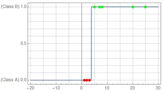
and then solve for the minimum cost, I got a good solution for W with a good fit as shown in the following picture:
Now I am trying to understand the Cost function given by:
\begin{align} J(W)= -\frac{1}{m}\sum_{i=1}^m ( y_{i}log(h( x_{i} ))+(1- y_{i} )(1-log(h( x_{i} )) ) \end{align}
When I visualize this function to see if it is convex or not I just got a weird shape with no convexity. Moreover, when I minimize it to get the values of W I got values for W which results in a bad fit for the data. Also every time I minimize the loss function with different initial values of W I always got different results for W.
Can you please let me know what did I do wrong to get these results?
I would like to see a 3D plot of the Cost function if possible to see the convexity of the Cost function.
Update
This is what I did: I prepared the data and prepared the h and Sigh functions as follows:
XY={{1, 1, 0}, {1, 2, 0}, {1, 3, 0}, {1, 5, 1}, {1, 7, 1}, {1, 8, 1},
    {1,20, 1}, {1, 25, 1}};
m=Length[XY];
   ClearAll[h, Sig, Sigh]
    h[x0 : 1, x_] = {x0, x}.{w0, w1}
    Sig[z_] = 1/(1 + E^-z)
    Sigh[x0 : 1, x_] = Sig[h[1, x]]
Then I prepared the cost function as follows:
ClearAll[Costfun]
Costfun[x0 : 1, x_,y_] = -y Log[Sigh[x0, x]] - (1 - y) (1 - Log[Sigh[x0, x]])
J[w0_, w1_] = 1/m Total[Costfun @@@ XY]
This is what I got (the plot is also included)

When I minimize the cost function I could not get correct values of W and this the fitting answer:


