Least Squares removing first $k$ observations Woodbury formula?

Question

Given the matrix $X_{n,p}$ from the least squares problem $$ \mathbf{X} \cdot \mathbf{\beta} = z $$

Where the normal equation is:

$$ \mathbf{\hat{\beta}} = \left(\mathbf{X}^T \mathbf{X}\right)^{-1} \mathbf{X}^T z $$

I was very happy when I found the existence of the Woodbury matrix identity unfortunantly I am struggling to use it (don't know if it's possible) for my problem.
$$ {(A+UCV)}^{-1}=A^{-1}-A^{-1}U{(C^{-1}+VA^{-1}U)}^{-1}VA^{-1} $$

The Problem

I want to compute a new $(X^TX)^{-1}$ after removing the first $k$ rows of $X$. I heard maybe it's called the leave-one-out (k-out?) statistics.

I found that for the my case the Woodbury formula is something like: $$ {((X^TX)+UCV)}^{-1}=(X^TX)^{-1}-(X^TX)^{-1}U{(C^{-1}+V(X^TX)^{-1}U)}^{-1}V(X^TX)^{-1} $$ where $+UCV$ should somehow subtract the first $k$ rows.

If someone can give some help or point to some direction or references.

Answer 1

You've basically laid out the key facts, I think you just need a hint on how to fit them all together. Here's a quick-and-dirty overview.

I think it's easier to see how to accomplish your goal if you build up from the Sherman-Morrison formula, which is just a special case of the Woodbury matrix identity. The Sherman-Morrison formula is a rank-1 update, while the Woodbury identity is a rank-$r$ update.

We have a matrix $X_{n \times p}$ with $n$ samples/observations of $p$ variables/features and $X$ is full rank. The product $X^\top X$ can be viewed as a sum of outer products. Denote $x_j$ the $j$th column of $X^\top$ (i.e. the transpose of the $j$th row of $X$). Suppose we leave out one row $k$. We have

$$ \begin{align} X^\top X &= \sum_j x_j x_j^\top \\ &= x_k x_k^\top + \sum_{j\neq k} x_j x_j^\top \\ X^\top X - x_k x_k^\top &= \sum_{j\neq k} x_j x_j^\top. \end{align} $$

Relating this to the Sherman-Morrison formula can be done by inspection. Sherman-Morrison gives us $$ (A + uv^\top)^{-1} = A^{-1} - \frac{A^{-1}uv^\top A^{-1}}{1+v^\top A^{-1} u}, $$

so we just need to make appropriate substitutions:

$$ \begin{align} A &= X^\top X \\ u &= -x_k \\ v^\top &= x_k^\top. \end{align} $$

And of course we can repeat this for $r > 1$ indices and then we are splitting $A=X^\top X$ into the sum of two non-empty sets of outer products, $k\in \mathcal{S}$ and its complement. This leads us to the Woodbury identity, because now we have a rank-$r$ update to $A$. (Naturally, we can't leave out too many rows because then we have non-invertible matrix problems, and the procedure will blow up if the "denominator" is too close to 0, signaling that removing these rows is causing the matrix to become ill-conditioned.)

So the Woodbury identity will use

$$\begin{aligned} C &= I_{r\times r}\\ U &= -X_{k\in\mathcal{S}}^\top \\ V &= X_{k\in\mathcal{S}}. \end{aligned}$$

One caveat here is that we haven't characterized the loss of precision incurred by using floating-point arithmetic. Before implementing this in code, I would recommend studying the numerical conditioning of this procedure.

A colleague observes that eventually, for $r=|\mathcal{S}|$ too large, this becomes more expensive than the original problem. A better alternative is to form a QR factorization. This procedure is faster and more accurate and has its own update capabilities. I believe this is outlined in Golub & van Loan but I don't have my copy handy.

Answer 2

Over here and here, the leave-one-out (LOOCV) formula uses Sherman-Morrison formula in its derivation. Deriving the leave-$k$-out would require the general formula by Woodbury, as you have suspected.

Here I use subscript $k$ as the indices for the rows to be left out from the training set, $(k)$ as the whole vector or matrix without the rows from $k$, and $[k]$ for submatrix containing only rows and columns from $k$. For convenience, the following matrices are defined $$ \begin{aligned} A &= X^TX \\ A_{(k)} &= X_{(k)}^TX_{(k)} \\ A_k &= X_k^TX_k \\ H &= XA^{-1}X^T \\ H_{[k]} &= X_kA^{-1}X_k^T \end{aligned} $$ $H$ is the so-called hat matrix, while $H_{[k]}$ is a submatrix of $H$. The original residual and the individual leave-$k$ out errors are described by $$ \begin{align} e_k&=z_k-X_k\hat\beta \\ e_{(k)}&=z_k-X_k\hat\beta_{(k)}\tag{1}\label{ek} \end{align} $$ where $$ \hat\beta_{(k)}=A_{(k)}^{-1}X_{(k)}^Tz_{(k)}\tag{2}\label{beta1} $$ We have the following identities $$ \begin{align} A_{(k)}=A-A_k \\ X_{(k)}^Tz_{(k)}=X^Tz-X_k^Tz_k \tag{3}\label{Xzk} \end{align} $$ From Woodbury identity we have the following $$ \begin{aligned} A_{(k)}^{-1}&=A^{-1}+A^{-1}X_k^T(I-X_k^TA^{-1}X_k)^{-1}X_kA^{-1}\\ &=A^{-1}+A^{-1}X_k^T(I-H_{[k]})^{-1}X_kA^{-1} \end{aligned} $$ Left multiplying $X_k$ gives us $$ \begin{aligned} X_kA_{(k)}^{-1}&=X_kA^{-1}+H_{[k]}(I-H_{[k]})^{-1}X_kA^{-1} \\ &=(I-H_{[k]})(I-H_{[k]})^{-1}X_kA^{-1}+H_{[k]}(I-H_{[k]})^{-1}X_kA^{-1} \\ &=(I-H_{[k]})^{-1}X_kA^{-1} \end{aligned} $$

Substituting $\eqref{Xzk}$ into $\eqref{beta1}$, we have from the above equation $$ \begin{aligned} X_k\hat\beta_{(k)}&=(I-H_{[k]})^{-1}X_kA^{-1}(X^Tz-X_k^Tz_k) \\ &= (I-H_{[k]})^{-1}(X_k\hat\beta - H_{[k]}z_k) \\ &= (I-H_{[k]})^{-1}(X_k\hat\beta - H_{[k]}z_k) \end{aligned} $$ This is finally inserted into the leave out formula $\eqref{ek}$ to get $$ \begin{aligned} e_{(k)} &= z_k-(I-H_{[k]})^{-1}(X_k\hat\beta - H_{[k]}z_k) \\ &= (I-H_{[k]})^{-1}\left[(I-H_{[k]})z_k-X_k\hat\beta+H_{[k]}z_k\right]\\ &= (I-H_{[k]})^{-1}(z_k-X_k\hat\beta) \\ &= (I-H_{[k]})^{-1}e_k \end{aligned} $$

which can be calculated by solving the following matrix equation to avoid the costly matrix inversion

$$ (I-H_{[k]})e_{(k)} = e_k $$ Unlike the LOOCV formula which had only scalars, solving the above may not be as cheap, depending on the size of $k$.

---

Extra note regarding $H_{[k]}$: $H$ can be very big. If you have $n$ points, the size is $n\times n$. Fortunately, you don't need the whole matrix to calculate the submatrix. If $\hat\beta$ is written as follows $$ \begin{aligned} \hat\beta &= Mz \\ M &= A^{-1}X^T \\ \end{aligned} $$ Then $M$ is typically determined by solving the following system $$ AM = X^T $$ The size of $B$ is $n\times m$, where $m$ is the number of bases. From here you can compute $$ H_{[k]} = X_{k}M_k $$ where $M_k$ are the columns from $M$ with the indices in $k$.

Another method is to use eigendecomposition on $X^TX$

$$ X^TX = PDP^T $$

so that its inverse can calculated as

$$ (X^TX)^{-1} = PD^{-1}P^T $$

Defining $Q=XP$, and $Q_{[k]}$ its $k$ rows, the hat matrix and its partial submatrix can be calculated as

$$ \begin{aligned} H &= XPD^{-1}P^TX^T = QD^{-1}Q^T \\ H_{[k]} &= Q_{[k]}D^{-1}Q_{[k]}^T \end{aligned} $$

Of course, calculating eigendecomposition can still be expensive, and so is solving for $e_{(k)}$. Therefore, this method is only worthwhile if the number of folds is large enough compared to the data points. If the data is large, it might be better to stick with the naive method for your typical 10-fold CV.

Here are some plots comparing the two approaches, for several folds and design matrix sizes.

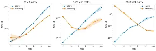
(The code for the benchmark can be found here)