Combining customized contrasts + nested ANOVA (?)

Question

I would like to get some advice on running a customized contrast analysis. I have looked at a few vignettes and I think I get the basic idea, but I'm not sure how to adapt them for my purpose.

To make things simple, let's just say that in this survey, people rated on a scale how much they want to visit cities in the east coast and west coast of the US. So a response like "New York, 10" means "I would very much love to visit New York" and "Seattle, 4" means "I don't really want to go to Seattle".

This dataset was collected in order to test the following three (competing) hypotheses.

I) Ratings for east coast cities > Ratings for west coast cities.

II) Ratings for east coast cities are comparable to each other. (New York = Boston = DC and so on. No claim about west coast cities.)

III) New York > all other cities.

I have two main questions.

1) I understand that hypotheses I and III can be coded as contrasts (non-orthogonal ones) and run in a single regression. But how do I include Hypothesis II in the same contrast analysis? (I'm assuming I should test all of them at once.)

If a contrast analysis isn't appropriate, what should I use? Some kind of ordinal ANOVA for the relevant cities? Edit: I did some Googling and found that a nested ANOVA might be suitable for Hypothesis II, but I'm not sure.

Are there any packages or vignettes I should use? I am hoping to run an ordinal analysis if that's helpful.

2) In the vignettes I saw, the output of a regression with contrasts indicate whether it is significant (t and p values), but not the direction of the contrast. But Hypotheses I and III are basically one-tailed hypotheses. How can I check for that?

Answer 1

At the time of writing, this is a very software-heavy answer. The following is R code, relying on the emmeans package to analysis custom contrasts for a model fit with the ordinal package. I suspect that emmeans will properly handle custom contrasts for supported models even if the design is more complex.

One thing to note here is that the classic way to analyze custom contrasts in R is with aov that limits the number of contrasts to the degrees of freedom in the e.g. treatment effect. However, emmeans and multcomp allow for any number of custom contrasts, and often a p value correction is applied to account for the multiple hypothesis tests.

Sources, with the caveat that I am the author of these webpages:

http://rcompanion.org/rcompanion/h_01.html

http://rcompanion.org/handbook/G_07.html

### Install packages ###
if(!require(ordinal)){install.packages("ordinal")}
if(!require(car)){install.packages("car")}
if(!require(RVAideMemoire)){install.packages("RVAideMemoire")}
if(!require(emmeans)){install.packages("emmeans")}
###                  ###

Input = ("
City           Response
 NY             4
 NY             5
 NY             6
 Boston         4
 Boston         5
 Boston         6
 DC             7
 DC             9
 DC            10

 Seattle        1
 Seattle        2
 Seattle        3
 SantaCruz      1
 SantaCruz      2
 SantaCruz      2
 Oxnard         1
 Oxnard         2
 Oxnard         4
")

Data = read.table(textConnection(Input),header=TRUE)


### Specify the order of factor levels. Otherwise R will alphabetize them.

Data$City = factor(Data$City, levels=unique(Data$City))


Data$Response = factor(Data$Response, ordered=TRUE)


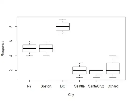
boxplot(Response ~ City,
        data = Data,
        ylab="Response",
        xlab="City")

###  You need to look at order of factor levels to determine the contrasts

levels(Data$City)

   ### "NY"        "Boston"    "DC"        "Seattle"   "SantaCruz" "Oxnard"

library(ordinal)

model = clm(Response ~ City, data = Data, threshold="equidistant")

   ### Normally you don't need threshold="equidistant"

library(car)

library(RVAideMemoire)

Anova(model,
      type = "II")

  ### Note that you shouldn't use car::Anova with `ordinal` models,
  ###  unless you use the modification in the `RVAideMemoire` package. 


library(emmeans)

em = emmeans(model, ~ City)


### Hypothesis I

Contrasts = list(East_vs_West = c(1,  1,  1,  -1,  -1,  -1))

   ### The column names match the order of levels of the treatment variable
   ### The coefficients of each row sum to 0

contrast(em, Contrasts, adjust="sidak")

   ### contrast     estimate   SE  df z.ratio p.value
   ### East_vs_West     23.4 6.03 Inf 3.878   0.0001 

   ### estimate is sided.  That is, it can be negative or positive.
   ### Here, obviously, East has higher values than West, and the estimate
   ###  is positive.

   ### For a one sided test, I guess you should just divide the p-value by two.

### Hypothesis II

Contrasts = list(NY_vs_Boston = c( 1, -1,  0,  0,  0,  0),
                 Boston_vs_DC = c( 0,  1, -1,  0,  0,  0),
                 DC_vs_NY     = c(-1,  0,  1,  0,  0,  0))

### Do omnibus test for differences among East Coast cities

Test = contrast(em, Contrasts)

test(Test, joint=TRUE)

   ### df1 df2 F.ratio p.value note
   ###   2 Inf   4.809 0.0082   d  
   ###
   ### d: df1 reduced due to linear dependence

### Look at pairwise comparisons of East Coast cities

contrast(em, Contrasts, adjust="sidak")

   ### contrast     estimate   SE  df z.ratio p.value
   ### NY_vs_Boston     0.00 1.49 Inf  0.000  1.0000 
   ### Boston_vs_DC    -5.78 2.01 Inf -2.881  0.0118 
   ### DC_vs_NY         5.78 2.01 Inf  2.881  0.0118 
   ###
   ### P value adjustment: sidak method for 3 tests 

## Hypothesis III

Contrasts = list(NY_vs_AllElse = c( 1, -1/5, -1/5, -1/5, -1/5, -1/5))

contrast(em, Contrasts, adjust="sidak")

   ###  contrast      estimate   SE  df z.ratio p.value
   ###  NY_vs_AllElse     2.36 1.28 Inf 1.841   0.0657