Modeling trends with Gaussian Processes

Question

I am trying to use Gaussian Process Regression to model data that has a clear upward rising trend. Here is a basic plot of the data -

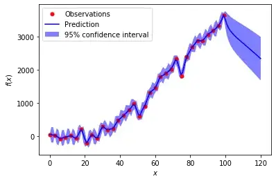
The most well-known example of the flexibility of GPs in such problems is shown in the modeling of Mauna Loa CO2 data, examples of which are shown both on the sklearn page and the book "Gaussian processes for machine learning" by Rasmussen. Here is a figure of the fitted model (and predictions) from the sklearn page

However, despite trying various different types of kernels and hyperparameters, I find it hard to model the trend, especially when the GP encounters data from an unseen region.

For example, this code snippet produces the following image -

gp = GaussianProcessRegressor(kernel=kernel,n_restarts_optimizer=100,alpha=1)
gp.fit(x,y)
testPoints = np.linspace(0,120,120)
yPred,sigma = gp.predict(testPoints.reshape(-1,1),return_std=True)
print("Log-marginal-likelihood: %.3f"% gp.log_marginal_likelihood_value_)
plt.figure()
plt.plot(x, y, 'r:')
plt.plot(x, y, 'r.', markersize=10, label=u'Observations')
plt.plot(testPoints, yPred, 'b-', label=u'Prediction')
plt.fill(np.concatenate([testPoints, testPoints[::-1]]),
         np.concatenate([yPred - 1.9600 * sigma,
                        (yPred + 1.9600 * sigma)[::-1]]),
         alpha=.5, fc='b', ec='None', label='95% confidence interval')
plt.xlabel('$x$')
plt.ylabel('$f(x)$')
plt.legend(loc='upper left')
plt.show()

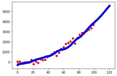
In order to model the obvious trend outside the 'seen' region in data, one possible solution is illustrated in a Cross Validated post here, which illustrates the benefit of regression-kriging --- essentially learning a polynomial regression model to capture the trend and using a GP model for the residuals. This code snippet for the data shown above yields the following fit (for the regression model) -

from sklearn.preprocessing import PolynomialFeatures
from sklearn import linear_model

poly = PolynomialFeatures(degree=2)
x_ = poly.fit_transform(x)
lm = linear_model.LinearRegression()
lm.fit(x_,y)
yPred = lm.predict(x_)
plt.figure()
plt.scatter(x,yPred,color='b',label='predictions')
plt.scatter(x,y,color='r',label='data')

The following is the result for the combined regression model and a gp fit to the residuals

Here are my questions -

1. Is it in practice, extremely difficult to model trends with GPs, especially when it entails prediction on a region of unseen data?

2. In such a case, is regression-kriging the most used method?

3. How does one calculate the confidence for such a model?

Answer 1

I extracted data from the scatter plot and ran it through the "function finder" on my open source Python zunzun.com curve fitting web site. It fit the data to 291 non-linear and 16 linear equations with 3 or less parameters, using a genetic algorithm to estimate initial parameters for the non-linear equations. The idea was to find the simplest smooth curve that gives a reasonably good fit, as that should both interpolate and extrapolate well.

Here is the top result, an inverted offset exponential equation "y = a * exp(b/(x+c))" with parameters a = 1.4271049053537125E+04, b = -1.3705804811393989E+02, and c = 1.2110000000070614E-01 yielding RMSE = 150.2 and R-squared = 0.984. I have extended the plot scaling to the right in order to display potential extrapolation.