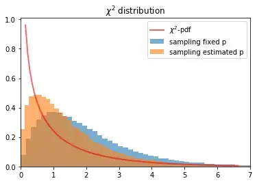
For a better understanding of a $\chi^2$-test (and teaching), I want to make an MC approximation for the $\chi^2$-distribution on a simple example (2x2 contingency table). This is a typical situation for an independence test:
Assume we have two binary variables X and Y and we measure n-times an (X,Y)-pair. The number of observed X=0 is fixed, e.g. 400 and the number of observed X=1 is also fixed, e.g. 600. So, we have 1000 observations.
We want to test for independence. The data can be summarized in a table, e.g. we observe:
 |     || Y=0 | Y=1 ||   |
 ---------------------------
 | X=0 || 350  |  50  || 400  |
 | X=1 || 250  |  350 || 600  |
 |     ||      |      || 1000 |
To my knowledge, we can use Pearson $\chi^2$ test for independence with the number of degrees of freedom = 1.
Now we simulate the situation:
t=10 # make the cell entries larger
data = np.array([[35,5],[25,35]])*t # not directly use in the simulation

# p(Y) estimated from data:
p_ = lambda d: (d.sum(axis=0))/d.sum()


#### simulation

def simulate_data(p, n1, n2):
    a = np.random.binomial(n=n1, p=p).reshape(1,2)
    b = np.random.binomial(n=n2, p=p).reshape(1,2)
    return np.concatenate((a,b),axis=0)

def get_expectation(p, n1, n2):
    a = (p*n1).reshape(1,2)
    b = (p*n2).reshape(1,2)
    return np.concatenate((a,b),axis=0)

sample_distribution_fix = []
sample_distribution_estimated = []


p = np.array([0.6, 0.4]) # assume that this is the true p(Y)=p(Y|X (independent of X)

sim_expected_fix = get_expectation(p, 40*t, 60*t)

for i in range(nb_simulations):
    sim_data = simulate_data(p, 40*t, 60*t)

    # fix p
    sample_distribution_fix.append( ((sim_data-sim_expected_fix)**2/sim_expected_fix).sum() )

    # p estimated from the data / reduces the degrees-of-freedom for the test?
    sim_expected = get_expectation(p_(sim_data), 40*t, 60*t)#
    sample_distribution_estimated.append( ((sim_data-sim_expected)**2/sim_expected).sum() )

# plot the sample distributions

df=1
x = np.linspace(scipy.stats.chi2.ppf(0.3, df), scipy.stats.chi2.ppf(0.99, df), 100)
plt.plot(x, scipy.stats.chi2.pdf(x, df), 'r-', lw=2, alpha=0.6, label='$\chi^2$-pdf')
plt.hist(sample_distribution_fix, bins=100, density=True, label='sampling fixed p', alpha=0.6)
plt.hist(sample_distribution_estimated, bins=100, density=True, label='sampling estimated p', alpha=0.6)
plt.xlim(0,7)
plt.title("$\chi^2$ distribution")
plt.legend();
Note: There are two simulations. One with fixed p(Y) and. The other estimate p(Y) from the corresponding sample. This is the situation we have in practice (this reduces the degrees of freedom: -1).
If the row sum and the column sum is fixed (simulated with a hypergeometric simulation) I get the expected $\chi^2$-distribution by MC. However, this is not the data generating process. Note: Here, the constraint enforces that the estimated $p(Y)$ is the same as the true $p(Y)$. So, the simulation becomes much easier.
# https://en.wikipedia.org/wiki/Hypergeometric_distribution#Working_example
nb_simulations=100000

s00 = np.random.hypergeometric(ngood=40*t, nbad=60*t, nsample=60*t, size=nb_simulations)
s = np.ndarray((nb_simulations, 2, 2))
s[:,0,0] = s00
s[:,0,1] = 40*t-s00
s[:,1,0] = 60*t-s00
s[:,1,1] = 60*t-s[:,1,0]
sample_distribution = ((s - expected)**2/expected).sum(axis=1).sum(axis=1)
So, I have the following questions:
- Is the assumption wrong, that we can use the $\chi^2$ test for the example above?
- Is there an issue with the sampling (using two binominal distributions)? Or why can I not reproduce the $\chi^2$-distribution by MC?
Thanks.
P.S.: (5.12.2019)
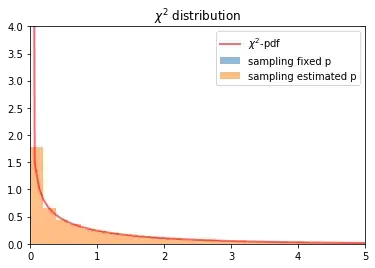
Thanks, it was a bug in simulate_data_binominal. The correct way to simulate is:
def simulate_data_binominal(p, n1, n2, px=None):
    a = np.random.binomial(n=n1, p=p[1])
    b = np.random.binomial(n=n2, p=p[1])
    return np.array([[n1-a,a],[n2-b,b]])
Now the simulation looks good:


