2

One of the conditions to use statistical inference, when estimating the proportion of a population based on the sample proportion, is that:

The data's individual observations have to display normality. This can be verified mathematically with the following definition:

Let $\displaystyle n$ be the sample size of a given random sample and let $\displaystyle {\hat {p}}$ be its sample proportion. If $\displaystyle n{\hat {p}}\geq 10$ and $\displaystyle n(1-{\hat {p}})\geq 10$, then the data's individual observations display normality.

In other source, it says that the sample size $n \ge 30$, which

this rule-of-thumb was developed by having a computer do what are called “Monte Carlo simulations”

So far, I haven't found a source that formalize any of these assumptions.

Could someone provide some references (articles, books) about this?

Kazh
  • 41
  • 8
  • 2
    It seems you may be dealing with two rough rules of thumb, each for applying a different method. Suggest you say more about your data and objectives. Then maybe we can give suggestions what method to use. – BruceET Nov 22 '19 at 23:07
  • 2
    The rules of thumb relating to proportions and sample means more generally that you're talking about were around long before simulation was a widely available tool. I doubt the assertion about simulation that you quote is true (that it originates by doing simulation), since it was around too early for that. You *can*, however, use simulation to investigate the $n\geq 30$ claim about sample means (and easily show it to be [false](https://stats.stackexchange.com/a/437379/805)). The usual rule of thumb for proportions would take $p$ into account, but again it predates the existence of computers. – Glen_b Nov 23 '19 at 02:17
  • @BruceET The point of the question is where these assumptions come from, rather than use them directly. – Kazh Nov 25 '19 at 10:07
  • Thanks for clarification. On [Wikipedia](https://en.wikipedia.org/wiki/Binomial_distribution) under '8.6. Normal Approx' you can find the rationale for the first rule (for normal aprx to binomial) along with other "rules of thumb" and some proofs. I hope to find time soon to illustrate with Answer. // As far as I can determine, the second rule (for normal aprx to Student's t) originated by observing that 2-sided 95% CIs and tests at 5% level for normal use $1.96≈2.0$ while t tests and CIs with df $=29$ use $2.0452≈2.0.$ Seems from there, many unwarranted 'rules of 30' proliferated. – BruceET Nov 25 '19 at 21:00
  • Ahh, so with >29 DoF using the Student's t, it's possible to get a rather good approximation of $95%$ CI, right? – Kazh Nov 25 '19 at 21:22
  • That's the simple version. Caveats: (1) If you're using 99% CI/1% level or anything else far from 95%/5%, then $n = 30$ is _nowhere near_ the right sample size. (2) If you're using software then use 'normal' procedures only when $\sigma$ is known (program will ask for known $\sigma)$ and use t procedures when $\sigma$ is estimated by $S.$ – BruceET Nov 25 '19 at 21:28
  • For 99% CI or 1% level, the "magic" number is around $n = 66.$ In R: `qnorm(.995)` returns 2.576 (aprx 2.6) and `qt(.995, 65)` retirms 2.654 (aprx 2.6). // Unfortunately, this gets conflated with the size of $n$ for which CLT gives $\bar X$ aprx normal. Another issue entirely. For uniform data that's about $n = 12$ and for exponential data $n = 100$ is not always sufficient. – BruceET Nov 25 '19 at 21:42
  • I will check that question. – Kazh Nov 26 '19 at 14:37
  • Yes, I think that question solves part of the problem. I could even add some references as an answer. – Kazh Nov 26 '19 at 14:48

3 Answers3

3

This rule-of-thumb is meaningless without specification of further details

I remember this same assertion being bandied around when I was first learning statistics, and really, it is meaningless without some specification of the conditions of assessing the approximation. The classical CLT applies to any underlying sequence of random variables that are IID from some distribution with a finite variance. This wide scope allows consideration of a huge number of possible underlying distributions, which vary substantially in how close they already are to the normal distribution (i.e., how good the accuracy is when $n=1$).

In order to specify a minimum required number of data points for "good approximation" by the normal distribution (even undertaking a simulation study or other analysis) you would need to specify two things:

  • How different to the normal distribution is the underlying distribution of the data?

  • How close to the normal distribution is "good enough" for approximation purposes?

Any attempt to formalise a rule-of-thumb for this approximation would need to specify these two things, and then show that the specified number of data points achieves the specified minimum level of accuracy for underlying data coming from the specified distribution.

Depending on how you specify the above two things, the minimum number of data points in the resulting "rule of thumb" will be different. If the underlying data is already close in shape to a normal distribution then the number of data points required for "good" approximation" will be lower; if the underlying data is substantially different in shape to a normal distribution then the number of data points required for "good approximation" will be higher. Similarly, if "good approximation" requires a very small "distance" from the normal distribution then the number of data points required for "good" approximation" will be higher; if "good approximation" is taken a bit more liberally, as allowing a higher "distance" from the normal distribution, then the number of data points required for "good" approximation" will be lower.

Ben
  • 91,027
  • 3
  • 150
  • 376
1

One quote I like to bring up about the greater than 30 rule for the Central Limit Theorem (implying normality) is from Rand Wilcox, 2017, Modern Statistics for the Social and Behavioral Sciences. Section 7.3.4.

Three Modern Insights Regarding Methods for Comparing Means

There have been three modern insights regarding methods for comparing means, each of which has already been described. But these insights are of such fundamental importance that it is worth summarizing them here.

• Resorting to the central limit theorem in order to justify the normality assumption can be highly unsatisfactory when working with means. Under general conditions, hundreds of observations might be needed to get reasonably accurate confidence intervals and good control over the probability of a Type I error. Or in the context of Tukey's three-decision rule, hundreds of observations might be needed to be reasonably certain which group has the largest mean. When using Student's T, rather than Welch's test, concerns arise regardless of how large the sample sizes might be.

• Practical concerns about heteroscedasticity (unequal variances) have been found to much more serious than once thought. All indications are that it is generally better to use a method that allows unequal variances.

• When comparing means, power can be very low relative to other methods that might be used. Both differences in skewness and outliers can result in relatively low power. Even if no outliers are found, differences in skewness might create practical problems. Certainly there are exceptions. But all indications are that it is prudent not to assume that these concerns can be ignored.

Despite the negative features just listed, there is one positive feature of Student's T is worth stressing. If the groups being compared do not differ in any manner, meaning that they have identical distributions, so in particular the groups have equal means, equal variances, and the same amount of skewness, Student's T appears to control the probability of a Type I error reasonably well under nonnormality. That is, when Student's T rejects, it is reasonable to conclude that the groups differ in some manner, but the nature of the difference, or the main reason Student's T rejected, is unclear. Also note that from the point of view of Tukey's three-decision rule, testing and rejecting the hypothesis of identical distributions is not very interesting.

Sal Mangiafico
  • 7,128
  • 2
  • 10
  • 24
1

Illustrations of previous comments.

Normal approximation to binomial.

A commonly used rule of thumb is that $np > K$ and $n(1-p) > K$ for some $K.$ In your question, $K = 10,$ but values $K = 5, 9, 20$ are also commonly quoted. The purposes of this and other 'rules of thumb' are to use a normal approximation only when the binomial distribution at hand has $n$ large enough for the CLT to have some effect, for $p$ to be 'relatively' close to $1/2$ so that the binomial is not too badly skewed, and to make sure that the approximating normal distribution puts almost all of its probability between $0$ and $n.$ The hope is to approximate probabilities of events accurately to about two decimal places.

I will illustrate with $n = 60$ and $p = 0.1,$ a case that meets the rule you mention for $K = 5$ but not for $K = 10.$

So for $X \sim \mathsf{Binom}(n = 60, p = .1),$ let's evaluate $P(2 \le X \le 4) = P(1.5 < X < 4.5).$ The exact value $0.2571812$ is easily obtained in R statistical software, using the binomial PDF dbinom or the binomial CDF pbinom.

sum(dbinom(2:4, 60, .1))
[1] 0.2571812
diff(pbinom(c(1,4), 60, .1))
[1] 0.2571812

The 'best-fitting' normal distribution has $\mu = np = 6$ and $\sigma = \sqrt{np(1-p)} = 2.32379.$ Then the approximate value $0.2328988$ of the target probability, using the 'continuity correction' is obtained in R as follows:

mu = 6;  sg = 2.32379
diff(pnorm(c(1.5,4.5), mu, sg))
[1] 0.2328988

So we do not quite get the desired 2-place accuracy. You could get almost the same normal approximation by standardizing and using printed tables of the standard normal CDF, but that procedure often involves some minor rounding errors. The following figure shows that the 'best fitting' normal distribution is not exactly a good fit.

enter image description here

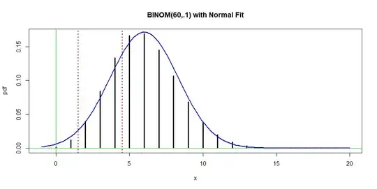
x = 0:20;  pdf = dbinom(x, 60, .1)
plot(x, pdf, type="h", lwd = 3, xlim= c(-1,20), 
     main="BINOM(60,.1) with Normal Fit")
 abline(h=0, col="green2");  abline(v=0, col="green2")
 abline(v = c(1.5,4.5), col="red", lwd=2, lty="dotted")
 curve(dnorm(x, mu, sg), add=T, lwd=2, col="blue")

For most practical purposes it is best to use software to compute an exact binomial probability.

Note: A skew-normal approximation. Generally speaking, the goals of the usual rules of thumb for successful use of the normal approximation to a binomial probability are based on avoiding cases where the relevant binomial distribution is too skewed for a good normal fit. By contrast, J. Pitman (1993): Probability, Springer, p106, seeks to accommodate to skewness in order to achieve a closer approximation, as follows. If $X \sim \mathsf{Binom}(n,p),$ with $\mu = np,$ and $\sigma = \sqrt{np(1-p)},$ then $$P(X \le b) \approx \Phi(z) - \frac 16 \frac{1-2p}{\sigma}(z^2 -1)\phi(z),$$ where $z = (b + .5 -\mu)/\sigma$ and $\Phi(\cdot)$ and $\phi(\cdot)$ are, respectively, the standard normal CDF and PDF. (A rationale is provided.)

In his example on the next page with $X \sim \mathsf{Binom}(100, .1),$ the exact binomial probability is $P(X \le 4) = 0.024$ and the usual normal approximation is $0.033,$ whereas the bias-adjusted normal approximation is $0.026,$ which is closer to the exact value.

pbinom(4, 100, .1)
[1] 0.02371108
pnorm(4.5, 10, 3)
[1] 0.03337651
pnorm(4.5, 10, 3) - (1 - .2)/18 * (z^2 - 1)*dnorm(z)
[1] 0.02557842

Normal approximation to Student's t distribution. The figure below shows that the distribution $\mathsf{T}(\nu = 30)$ [dotted red] is nearly $\mathsf{Norm}(0,1)$ [black]. At the resolution of this graph, it is difficult to distinguish between the two densities. Densities of t with degrees of freedom 5, 8, and 15 are also shown [blue, cyan, orange].

enter image description here

Tail probabilities are more difficult to discern on this graph. Quantiles .975 of standard normal (1.96) and of $\mathsf{T}(30)$ are both near $2.0.$ Many two-sided tests are done at the 5% level and many two-sided confidence intervals are at the 95% confidence level. This has given rise to the 'rule of thumb' that standard normal and $\mathsf{T}(30)$ are not essentially different for purposes of inference. However, for tests at the 1% level and CIs at the 99% level, the number of degrees of freedom for nearly matching .995 quantiles is much greater than 30.

qnorm(.975)
[1] 1.959964
qt(.975, 30)
[1] 2.042272

qnorm(.995)
[1] 2.575829  # rounds to 2.6
qt(.995, 70)
[1] 2.647905  # rounds to 2.6

The legendary robustness of the t test against non-normal data is another issue. I know of no sense in which a 'rule of 30' provides a useful general guide when to use t tests for non-normal data.

If we have two samples of size $n = 12$ from $\mathsf{Unif}(0,1)$ and $\mathsf{Unif}(.5,1.5),$ respectively, a Welch t test easily distinguishes between them, with power above 98%. (There are better tests for this.)

pv = replicate(10^6, t.test(runif(12),runif(12,.5,1.5))$p.val)
mean(pv < .05)
[1] 0.987446

Moreover, if we have two samples of size $n = 12$ from the same uniform distribution, then the rejection rate of a test at the nominal 5% level is truly about 5%. So for such uniform data it doesn't take sample sizes as large as 30 for the t test to give useful results.

pv = replicate(10^6, t.test(runif(12),runif(12))$p.val)
mean(pv < .05)
[1] 0.05116

By contrast, t tests would not give satisfactory results for samples of size 30 from exponential populations.

Note: This Q&A has relevant simulations in R.

BruceET
  • 47,896
  • 2
  • 28
  • 76