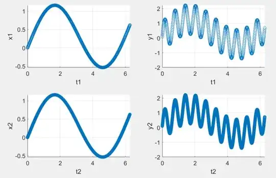
The setting. Let us assume I would like to perform Bayesian inference for a low-dimensional model on a large dataset, i.e., there are many more data points than there are parameters to identify. Let us moreover assume - as is always the case in practice - that the model is imperfect: it does not describe reality exactly.
The outcome. It is known that for many data points, the evidence introduced by the data often largely outweighs the influence of the prior. The posterior of the parameters will become more and more narrow with a growing number of data points, even if the model may not fit the data very well and no new information is gained from these new datapoints!
Example. We want to estimate the parameters $a$ and $b$ in the linear model $$ y = ax + b, $$ with priors $p(a)$ and $p(b)$ given, where $x(k)$ and $y(k)$ are discrete-time measurements of two slowly time-varying processes. $x(t)$ and $y(t)$ are approximately, but not exactly, related by the linear model given above: In "reality", $$ y = ax + b + c \cdot\sin(\omega t), $$ where the term $c\cdot\sin(\omega t)$ is not included in the regression model above and hence represents the model error / misspecification in this example.
Consider the following two test cases with different sampling rates ($f_2=10f_1$):
 The parameter estimates for both test cases are almost the same, but the estimated variances in case 2 are about one third of the variances in case 1. (Code + detailed results below).
Question. Intuitively, I would expect a "reasonable inference procedure" to yield the same result for both settings, including the variances: Essentially, no new information relevant to the given, low-dimensional model is gained from the additional samples in case 2. While I technically understand how it happens, this influence of the sampling rate / number of samples on the inference result appears undesired / defective. How can I fix this? To me, this appears to be an artifact of the inference procedure assuming the model to be perfect. Can I include some kind of "model uncertainty prior" to make the inference yield the same result in both cases, "recognizing" that no new information is gained?
Details on the example (Matlab).
t1 = 0:.01:2*pi; t2 = 0:.001:2*pi;
x = @(t) sin(t) + 0.1*t;
y = @(x, t) x + 0.1 + sin(10*t);
x1 = x(t1); x2 = x(t2);
y1 = y(x1, t1); y2 = y(x2, t2);

subplot(2, 2, 1);
scatter(t1, x1);
xlabel('t1'); ylabel('x1');
subplot(2, 2, 2);
scatter(t1, y1);
xlabel('t1'); ylabel('y1');
subplot(2, 2, 3);
scatter(t2, x2);
xlabel('t2'); ylabel('x2');
subplot(2, 2, 4);
scatter(t2, y2);
xlabel('t2'); ylabel('y2');

n_params = 1;
prior = bayeslm(n_params, 'ModelType', 'conjugate', 'Mu', [0, 0.5], 'V', eye(2));
prior.A = 0.001; prior.B = 0.001;
posterior1 = estimate(prior, x1', y1');
posterior2 = estimate(prior, x2', y2');
Outputs:
Method: Analytic posterior distributions
Number of observations: 629
Number of predictors:   2
Log marginal likelihood: -1316.96

           |  Mean     Std         CI95        Positive        Distribution
----------------------------------------------------------------------------------
 Intercept | 0.1099  0.0871  [-0.061,  0.281]    0.897   t (0.11, 0.09^2,6.3e+02)
 Beta      | 0.9679  0.1325  [ 0.708,  1.228]    1.000   t (0.97, 0.13^2,6.3e+02)
 Sigma2    | 3.6909  0.2088  [ 3.304,  4.122]    1.000   IG(314.50, 0.00086)


Method: Analytic posterior distributions
Number of observations: 6284
Number of predictors:   2
Log marginal likelihood: -8303.38

           |  Mean     Std         CI95        Positive        Distribution
----------------------------------------------------------------------------------
 Intercept | 0.1095  0.0130  [ 0.084,  0.135]    1.000   t (0.11, 0.01^2,6.3e+03)
 Beta      | 0.9698  0.0198  [ 0.931,  1.009]    1.000   t (0.97, 0.02^2,6.3e+03)
 Sigma2    | 0.8182  0.0146  [ 0.790,  0.847]    1.000   IG(3142.00, 0.00039)