Bias of overlap sampling

Question

Say I have a series $x_1, ...., x_N$ independently drawn from $Normal(0,1)$

Say I create sub-samples

$y_1 = x_1+..x_n$,
$y_2 = x_2+..x_{n+1}$,

$y_m = x_{N-n}+..x_N$,

I was expecting $std(\{y\}) = \sqrt(n) std(\{x\})$

where $std(\{y\})$ is the standard deviation of the set $y_1,...,y_m$. where $std(\{x\})$ is the standard deviation of the set $x_1,...,x_N$.

But this is not the case. Because of overlap sampling $std(\{y\}) < \sqrt(n) std(\{x\})$

If I performed non-overlapped sampling like

$z_1 = x_1+..x_n$,
$z_2 = x_{n+1}+..x_{2n}$,

$z_p = x_{pn+1}+..x_N$,

then I would get $std(\{z\}) = \sqrt(n) std(\{x\})$

here $std(\{z\})$ is the standard deviation of the set $z_1,...,z_p$.

My question: is there a theoritical estimate of the amount of bias for normal distribution ?

Thanks in advance

Answer 1

In order to be clear about what can be said, in the following analysis capital letters refer to random variables (not their realizations).

You have $N$ independent random variables $X_i$ with identical Normal$(0,1)$ distributions. From them you form $m$ new variables $Y_1=X_1+\cdots+X_n$ and so on. Very generally, you can form new variables out of old by choosing any coefficients $a_{ij}$ you like and set

$$Y_i = \sum_{k=1}^N a_{ik} X_k$$

for $i=1, 2, \ldots, m.$

The question asks about the variance of the "set" of $Y_i$ (its square root would be the standard deviation). I believe we have to understand that as referring to some multiple of the expression

$$\sum_{i=1}^m (Y_i - \bar Y)^2\tag{*}$$

where $\bar Y = (Y_1 + \cdots + Y_m)/m.$ (The usual multiples are $1/m$ and $1/(m-1).$ A constant multiple presents no problem, because ultimately it will just multiply the standard deviation.)

Let $\mathbb{A}=(a_{ik})$ be the $m\times N$ matrix of coefficients and let $\mathbb{P} = \mathbb{I}_m - \mathbf{1}^\prime \mathbf{1}$ be the matrix the removes the column means from $\mathbb A$ when multiplied (on the left). In these terms, $(*)$ is the quadratic form in the vector $\mathbf{X}=(X_1,X_2, \ldots, X_N)$ with matrix

$$\mathbb{Q} = \mathbb{A}^\prime \mathbb{P} \mathbb{A}.$$

Because $\mathbb Q$ is symmetric and positive-semidefinite, it can be diagonalized with an orthogonal transformation. This means we may express the form as

$$\sum_{i=1}^m (Y_i - \bar Y)^2\tag{*} = \sum_{j=1}^{N} \lambda_j Z_j^2$$

with all the $\lambda_j$ non-negative and, because (a) the $Z_j$ are linear combinations of the independent Normal variables $X_k$ and (b) these linear combinations are orthogonal, the $Z_j$ are independent standard Normal variables. Their squares $Z_j^2$ all have $\chi^2(1)$ distributions (by definition), exhibiting $(*)$ as a linear combination of independent $\chi^2(1)$ distributions. Its square root (multiplied by a suitable constant) gives the distribution of the sd of the $Y_i.$

---

Because a $\chi^2(1)$ distribution is a multiple of a $\Gamma(1/2)$ distribution, the analysis at https://stats.stackexchange.com/a/72486/919 shows there is no simple expression for it. Even in the case where $\mathbb A$ is given as in the question, all we can say generally is that $N-m$ of the $\lambda_j$ are nonzero and that their range increases as $N-m$ increases (precluding simple general approximations that assume the nonzero $\lambda_j$ are equal). It scarcely seems worthwhile to work out formulas for the $\lambda_j$ in terms of $N$ and $m,$ although surely that could be done.

The foregoing analysis does suggest the distribution might be approximated by some chi distribution (which governs the square root of a chi-squared variable). By matching moments of the chi-squared distributions (before taking square roots), the mean would be

$$\mu = \frac{1}{\sqrt{N-n}} \sum_i \lambda_i$$

and the variance would be

$$\sigma^2 = \frac{2}{N-n} \sum_i \lambda_i^2.$$

Therefore the approximating Gamma scale parameter would be

$$\theta = \frac{\mu}{\sigma^2}$$

and the shape parameter would be

$$k = \frac{\mu}{\theta} = \frac{\mu^2}{\sigma^2}.$$

The approximation is exact when $m=1$ and appears to work well for large $N$ and $n$ not close to $N/2.$ Here is an example for $N=39$ and $m=10:$

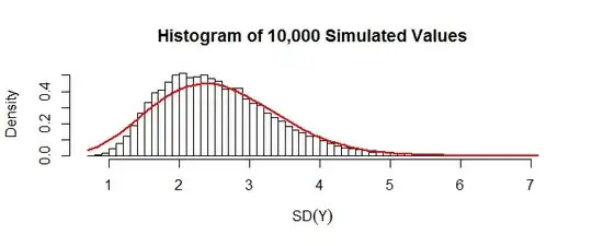
The red curve plots the density of the $\chi(2.200655, 1/17.80457)$ distribution (the parameters are shape and scale, respectively). Qualitatively this approximation is ok. When $N$ is five times larger (keeping $m=10$ as before), the approximation (now with a $\chi(13.70688, 1/9.449866)$ distribution) is excellent:

---

This R code creates a matrix $A:$

N <- 39*5
n <- 10
A <- outer(seq_len(N-n+1), seq_len(N), function(i,j) ifelse(i <= j & j < i+n, 1, 0))

A simulation of the standard deviations then is straightforward:

n.sim <- 1e4
X <- matrix(rnorm(n.sim * N), N)
Y <- A %*% X
S2 <- apply(Y, 2, sd)

Finding the eigenvalues $\lambda_i$ requires forming the matrix $\mathbb Q:$

m <- dim(A)[1]
P <- diag(rep(1,m)) - matrix(1/m, m, m)
Q <- t(A) %*% P %*% A
lambda <- zapsmall(eigen(Q, only.values=TRUE)$values)
lambda <- lambda[lambda > 0]

The last figure was constructed from the simulated SDs stored in S2 and eigenvalues stored in lambda:

mu <- sum(lambda) / sqrt(N-n)
sigma2 <- 2 * sum(lambda^2) / (N-n)
theta <- sigma2/mu
k <- mu/theta

hist(S2, freq=FALSE, breaks=50, xlab=expression(SD(Y)), 
     main="Histogram of 10,000 Simulated Values")
curve(2*x*sqrt(N-n)*dgamma(sqrt(N-n)*x^2, k, 1/theta), add=TRUE, col="Red", lwd=2)