What is the interpretation of the "C" parameter in the five parameters logistic curve?

Question

I'm using the following equation for the 5-parameters logistic curve: $$ y = A + \frac{D-A}{\Bigl(1+\exp\bigl(B(C-x)\bigr)\Bigr)^S} $$ What is the interpretation of the $C$ parameter?

I found some docs which say that it corresponds to the inflection point, some other docs which say that it corresponds to the $y$-value at the midpoint of the two asymptotes, as in the case $S=1$ (the case of the 4-parameters logistic curve).

But this is not true:

x <- seq(46, 53, length.out = 100)
A <- 30; D <- 100; B <- 5; C <- 50; S <- 10
y <- A + (D-A)/(1+exp(B*(C-x)))^S 
plot(x, y, type = "l")
abline(v = C, col = "red", lwd = 2)

Is there an interpretation of $C$?

score 3 · Accepted Answer · answered Nov 01 '19 at 13:18

$C$ is manifestly a location parameter.

It helps to understand that when $x$ and $y$ have a unit of measure, the choices of their origin and basic unit are essentially arbitrary. You can exploit that to make choices that simplify the formula and therefore reveal the essential shape of the curve.

Mathematically, this means you should rewrite the formula $y=f(x;\theta)$ in the form

$$\frac{y - \nu}{\tau} = f_0\left(\frac{x-\mu}{\sigma}; \theta^\prime\right)$$

where $\theta^\prime$ has four fewer parameters than $\theta=(A,B,C,D,S).$

In terms of the graph $\Gamma(f)=\{(x, f(x;\theta))\mid x\in \mathbb R\}$ this has the familiar geometric interpretation: the transformation of $x$ stretches the horizontal axis by $\sigma\gt 0$ and then shifts that axis by $\mu;$ the transformation of $y$ is the inverse of a rescaling by $\tau$ and shift of $\nu.$ Equivalently, on a plot of $\Gamma(f_0)$ simply relabel any ordinate $x$ as $\mu+x\sigma$ and any abscissa $y$ as $\nu + y\tau.$

This can usually be done by inspection. In the present case, the curve takes the form

$$y = f(x; (A,B,C,D,S))$$

which with simple algebraic manipulations can be written

$$\frac{y-\nu}{\tau} = \frac{y-A}{D-A} = \left(1 + \exp(-B(x-C))\right)^{-S} = \left(1 + \exp\left(-\frac{x-\mu}{\sigma}\right)\right)^{-S}$$

from which we can just read off the equations

$$\tau=D-A,\ \nu = A,\ \mu=C,\ \sigma=\frac{1}{B}$$

and identify the underlying shape as

$$f_0(z;S) = \left(1 + \exp(-z)\right)^{-S}.$$

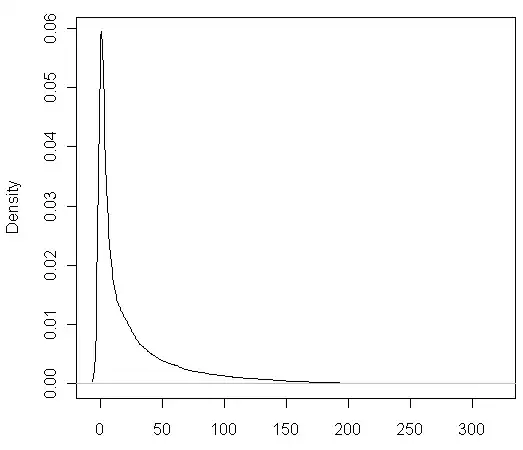
To understand these particular shapes, plot them on semi-log axes: that is, consider the graphs of $\log_2(y) = \log_2(f_0(x)) = -S\log_2(1 + \exp(-x)).$

Evidently $S$ is the value of $\log_2(y)$ when $z=0:$ that is, it establishes a logarithmic scale for $y$ by making the value of $f_0(0)$ equal to $S.$ Given this interpretation of $S,$ $\mu = C$ becomes meaningful as corresponding to the unique point where $\Gamma(f_0)$ equals $S.$

Thanks. I knew C is a location parameter. But I need a "nice" interpretation, short and suitable for non-statisticians, as in the case S=1. I accept your answer for the good work. — Stéphane Laurent, Nov 02 '19 at 10:31
There are many possible useful characterizations of $C.$ For instance, you could choose $f_0(z;S) = 2^S(1+\exp(-z))^{-S}-1,$ in which case $C$ is the intercept of $f_0.$ Of course this choice of $f_0$ changes the interpretations of $A$ and $D-A,$ suggesting you might want to reparameterize the family. — whuber, Nov 02 '19 at 13:21

score 2 · Answer 2 · answered Nov 01 '19 at 11:05

There's no direct interpretation of $C$.

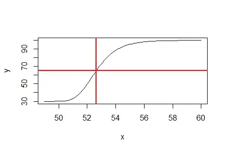
To get the value of $x$ corresponding to the midpoint between the two asymptotes, one solves an easy equation and one gets $$ xmid = C - \frac{\log\Bigl(2^{\frac{1}{S}}-1\Bigr)}{B}. $$

x <- seq(49, 60, length.out = 100)
A <- 30; D <- 100; B <- 1; C <- 50; S <- 10
y <- A + (D-A)/(1+exp(B*(C-x)))^S 
plot(x, y, type = "l")
xmid <- C - log(2^(1/S) - 1)/B
abline(v = xmid, col = "red", lwd = 2)
abline(h = (A+D)/2, col = "red", lwd = 2)

What is the interpretation of the "C" parameter in the five parameters logistic curve?

2 Answers2