1

I am collecting averages of scores between 1 and 5 on a customer satisfaction survey. Sample sizes are routinely less than 20 for shorter periods. (Over longer periods, this is not a problem, as the sample size increases sufficiently.)

The population mean is expected at 4.78, and the population standard deviation is estimated to be .6.

I would have loved to use a t-table with n-1 degrees of freedom to get the confidence interval for two or three standard deviations for the sampling distribution. Unfortunately, with a sample size of 20, both two and three standard deviations to the right extend beyond the range of possible scores, meaning that sample size isn't even approximately normally distributed, right?

I am more interested in the spread of the data to the left, but I don't want this to be thrown off from the spread of the data to the right.

How can I get the probability of scoring a certain amount below or above the mean in such a situation with such a sample size?
Mr. A
  • 171
  • 4
  • It seems odd that you're treating these apparently ordinal scores as numerical values. With a mean of 4.78, there's zero probability that someone scores 0.75 below the mean (they can only score a 4). Similarly, the probability that someone scores at least 0.8 below the mean is identical to the probability that they score at least 1.5 below the mean (both are between 3 and 4). A normal distribution isn't the right tool to describe an ordinal scale. – Nuclear Hoagie Sep 12 '19 at 13:22
  • @NuclearWang - It is possible to score below a 4. Possible raw scores are 1,2,3,4,5. But the scores are averaged. So if I had a sample of one 5 and one 1, the average score would be 3, 1 point below 4. It is not possible to go over 5 or below one, however. – Mr. A Sep 12 '19 at 13:26
  • Since your data is discreet and you mean value is near the upper end of the allowable ranges. you may want to consider using a bootstrap sampling technique to estimate the limits instead of the t-score. – Dave2e Sep 12 '19 at 13:36
  • @DaveT Tell me more? – Mr. A Sep 12 '19 at 13:53
  • Aside from bootstrapping (which is nice in being very straightforward) you may also compute a distribution more directly/exactly. Or at least, for a given categorical distrubution (probabilities of the different classes/scores) you should be able to compute, with an exact function, the sample distribution of the mean. And you can estimate that distribution with your data. – Sextus Empiricus Sep 12 '19 at 15:34
  • @Mr.A Ah, so your final score for each sample is an average among multiple 1-5 ratings, which makes your data more like a continuous variable, so my comment may not apply. My concern was that you were trying to model scores that could only be integer values from 1 to 5 - in that case, trying to assign probabilities to a score of 4.1 or 4.3 or 4.7 would be meaningless, since you can only ever be a 4 or 5 (so modeling between integers is pointless). – Nuclear Hoagie Sep 12 '19 at 20:34
  • @NuclearWang An average is just as discrete as a sum; you're just scaling the same distribution of values – Glen_b Sep 12 '19 at 21:51
  • @Glen_b Yes, an average of discrete numbers will be discrete, but it can be continuous "enough" to model with continuous distributions. The binomial distribution, for example, can be used to model success rate from a finite number trials, which can only take discrete values in intervals of 1/N. But as N grows large, the continuous normal distribution becomes a very good approximation for this discrete binomial distribution. If there are enough discrete scores for each sample, the distribution sample-wise averages over the whole population can be modeled with a continuous distribution. – Nuclear Hoagie Sep 13 '19 at 12:54
  • My point was simply that *averaging* is no better than *summing* as far as approach to normality goes. – Glen_b Sep 14 '19 at 03:15

3 Answers3

1

From Wikipedia: "In statistics, bootstrapping is any test or metric that relies on random sampling with replacement." See the Wikipedia article for the list of advantages and disadvantages. https://en.wikipedia.org/wiki/Bootstrapping_%28statistics%29

The basic procedure is to assume your sample of N individuals represents the distribution of the population.
Now sample your sample N times with replacement and calculate your test metric and record the results. Now repeat. The distribution of the test metric should now estimate the sample variation of the population. From estimate determine the confidence limits.

Example: You have sample of 10 people with the following scores (2, 3, 3, 3, 3, 4, 4, 4, 4, 5), mean 3.5
Now sample these scores with replacement 10 times and calculate a new mean.
Now repeat many times. Resulting in a list of values (3.7 3.6 3.6 3.2 3.7 3.5 …)
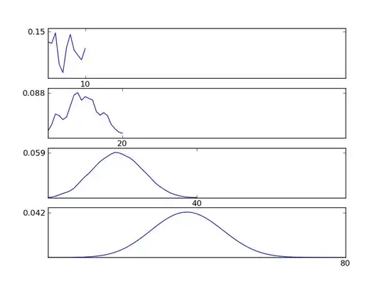
The distribution the calculated means is the distribution estimate. The histogram below is shown after 1000 resamples:
enter image description here

Dave2e
  • 1,441
  • 4
  • 14
  • 18
1

This sounds like a really good application for the multinomial distribution. Since the scores are ordinal (1 through 5), it doesn't make sense to treat them as numerical. That your proposed confidence intervals exceed the upper limit of 5 is a good sign that this is the case.

Instead, let's model the data as multinomial with 5 categories. An estimate for the multinomial parameter $\hat{\pi} = \left( \hat{\pi}_1, \hat{\pi}_2, \dots, \hat{\pi}_5 \right)$ is simply

$$ \hat{\pi}_j = \dfrac{1}{n} \sum_i \mathbb{I}(x_i=j) $$

Simply count up the number of times you observe a rating of 1, for example, and divide by the total sample size. This is your estimate for the probability that you observe a 1.

To estimate the probability we observe a score lower than some category, let's first estimate the odds of observing a category as opposed to all the others that precede it. We can use continuing ratio logins to do so

$$\hat{\theta}_j = \log\left(\dfrac{\hat{\pi}_j}{\sum_{i<j} \hat{\pi_i}}\right)$$

$\hat{\theta}_j$ is the estimate of the odds of falling in category $j$ as opposed to falling in any of the preceding $j-1$ categories. The variance of this estimator is given by

$$ \operatorname{Var}(\hat{\theta}_j) = \dfrac{1}{n} \left( \dfrac{1}{\sum_{i<j} \hat{\pi_i}} + \dfrac{1}{\hat{\pi}_j} \right) $$

This expression is found in chapter 2 of Lachin's "Biostatistical Research Methods" Second edition.

The logits are assumed to be asymptotically normal, which means we can apply the simple estimate + 1.96 the standard deviation. Then, we can transform the confidence interval back into the probability space to obtain the desired probability via an inverse logic transformation.

Demetri Pananos
  • 24,380
  • 1
  • 36
  • 94
0

As a general statement, the $t$-test is used when you're assuming that each sample comes from a population with an unknown mean and unknown standard deviation. You should consider whether you should model the samples as varying in both their mean and their standard deviation ($t$-test), or having a fixed standard deviation and varying mean ($z$-test).

However, the above doesn't apply in the case your discussing. Both tests assume that the underlying distribution is normal. Here, you have a multinomial distribution, but it's acting much like a binomial. If the population mean is 4.78, then the majority of responses are fives. (If all of the responses are fives and fours, then 78% are fives. If some of them are smaller then four, then the percentage of fives must be even higher.) Since the results are so dominated by fives, it can for many purposes be analyzed by simply dumping all the non-fives into one bucket, giving a binomial distribution, without losing much accuracy. Binomial distributions converge to normal somewhat slowly, and they are especially slow when the single-trial probability is far from 0.5, as is the case here. You should look into, rather than treating it as normal and trying to estimate the parameters of $\mu$ and $\sigma$, treating it as binomial and trying to estimate the single-trial probability $p$ that someone will give a five. You can find more information here: https://en.wikipedia.org/wiki/Binomial_proportion_confidence_interval

How can I get the probability of scoring a certain amount below or above the mean in such a situation with such a sample size?

If you mean the probability of a single person giving a particular score, that's not really something that you can derive from this sort of analysis. There's no reason to think that the probabilities of the different scores follow a normal, or any other standard, distribution. You'll just have to treat this as a four unknowns that you need to estimate.

Acccumulation
  • 3,688
  • 5
  • 11