2

I would like to see the convergence of an order statistic to its respective Extreme Value attractor by simulating with the Metropolis Hastings algorithm (I am self-studying MCMC algos). I was trying with a known case, the Normal maximum convergence to the Gumbel distribution. However I can't get a satisfactory result.

[EDIT following comment]

I'm simulating through the Metropolis Hastings the following random variable

$max(x_1, x_2, ...x_n)$ with each $N(0,1)$

according to Extreme Value Theory - Show: Normal to Gumbel it should converge to the Gumbel distribution

I'm trying to reach this result by sampling with the MH algorithm both the distribution of the maximum and the Gumbel random variable. The distribution of the maximum turns out to be completely off with respect to the Gumbel rv.

I'm computing the acceptance ratio in this way

$\alpha = \min\left(1,\frac{f(x_{proposed})}{f(x_{previous})} \frac{q(x_{previous}|x_{proposed})}{q(x_{proposed}|x_{previous})}\right)$

where $f$ is the density of the order statistic $f^{max}_n(x) = n f(x) F(x)^{n-1}$ and $q$ is the density of the proposal, in my case $N\left(\mu = x_{previous},10\right)$ (I chose this value for the variance to get an acceptance rate of about $10\%$) with $x_0 = 0$

[/EDIT]

I show it below along with the Python code (I attach it to allow to replicate my result)

import numpy as np
import matplotlib.pyplot as plt
import scipy.stats as st
def MH(func, numsample, cntsample):

    accepted_trials = []
    scale = 10

    floor = lambda x: 10e-14 if x < 10e-14 else x
    pdfproposal = lambda x, loc, scale: st.norm.cdf(x, loc = loc, scale = scale)
    qproposal = lambda loc, scale: np.random.normal(loc = loc, scale = scale)


    counter = 0

    for i in range(numsample):

        if i == 0:
            param_old = qproposal(loc = 0, scale = 1)

        param_new = qproposal(loc = param_old, scale = scale)

        alpha = min(1, func(param_new) / floor(func(param_old)) * \
                pdfproposal(param_old, param_new, scale) / floor(pdfproposal(param_new, param_old, scale)))


        u = np.random.uniform()                
        if alpha > u:
            accepted_trials.append(param_new)   
        param_old = param_new

        counter += 1

        print(counter, i, sep = ' ')
        if counter == cntsample:
            break

return accepted_trials

This is the code of my hand-written MH algorithm

n = 9 # distribution of the maximum for a sample size of 9 observation normally distributed
f = lambda x: st.norm.cdf(x)**n
g = lambda x: (f(x + 0.00001) - f(x))/ 0.00001
gumbelpdf = lambda x: np.exp(-x - np.exp(-x))
u = np.random.uniform(size = 50000)

accepted_trials_ordstat = MH(g, 200000, 50000)
accepted_trials_gumbel = MH(gumbelpdf, 200000, 50000)

Here I do feed it with the pdf (taking the numerical derivative makes no difference) of the maximum $f^{max}_n(x) = n f(x) F(x)^{n-1}$. Below the plots.

Comparing MH convergence to Gumbel

The blue line is the pdf MH-sampled of the order statistic, the orange line is the MH-sampled Gumbel distribution, the green line is Gumbel rv sampled directly with the inverse of cdf.

Playing with variance is of no help, actually the algorithm seems to be right, because if I compute $P(X \leq 0)$ with $F(x)$ of the maximum I get a value of 1.5% (it shrinks further if I increase $n$), while it's about 36% for the Gumbel. I am confused.
  • You're right, I added a section, hopefully it's clearer – Vittorio Apicella Sep 03 '19 at 23:58
  • Thanks for the edit, it definitely helps reduce the issues I raised. – Glen_b Sep 04 '19 at 00:03
  • If I was doing this exercise I'd be inclined to try to separate any issues with the approach to the Gumbel distribution family from issues relating to $a_n$ and $b_n$. In particular, I'd be wanting to look at something like a Q-Q plot - i.e. to plot the order statistics against $-\log(-\log(u_i))$ where $u_i$ is of the form $\frac{i-\alpha}{n+1-2\alpha}$. For large $n$ as you have, $\alpha=\frac12$ should be fine. – Glen_b Sep 04 '19 at 00:19
  • Also, can you clarify why you are using Metropolis-Hastings for this? – Glen_b Sep 04 '19 at 00:21
  • I was reading that MH could be used for sampling from any distribution, hence I chose something I have been interested for a long time, the distribution of this order statistic and see if it converged to the theoretical result. No other particular reason. – Vittorio Apicella Sep 04 '19 at 00:24
  • Sorry, I'm probably missing something. When I simulate the Gumbel rv with the quantile distribution ( $F^{-1}(u_i) = -\log\left(-\log\left(u_i \right)\right)$ ) (green line), I just pick random draws from the $U\left(0,1\right)$ just as I do for any other random variable. – Vittorio Apicella Sep 04 '19 at 00:28
  • I'm not referring to your simulation of the Gumbel but of the largest order statistic. Rather than simulate from the Gumbel and compare histograms (or anything else), first compare your blue distribution with what you'd expect - but rather than look at density, I'm suggesting you look at a QQ plot instead so that only the shape is considered (the location and scale parameters simply affecting the slope and intercept, which in turn only impacts the axis labels). – Glen_b Sep 04 '19 at 00:38
  • The idea in each of my suggestions (including those now deleted) is to look at things that will isolate particular issues from other kinds of issue.. e.g. if the code is correctly implementing the source information and the QQ plot is pretty linear then it must be an issue with $(a_n,b_n)$ (e.g. perhaps the $a_n$ and $b_n$ being interchanged -- some sources interchange their definitions relative to other sources -- or perhaps being incorrectly defined in some way). But if the QQ plot isn't linear, then the issue seems to be with convergence to the Gumbel, rather than with the $a_n$ and $b_n$ – Glen_b Sep 04 '19 at 00:41
  • The strategy is: when something doesn't work as expected, there's a host of potential places for there to be an issue. You then attempt a series of steps that will separate different kinds of problem. A divide-and-conquer strategy, where particular kinds of problem are ruled out or ruled in. Anything ruled out reduces the uncertainty about where to look for a problem. Anything ruled in focuses attention on that aspect. Hence the initial advice to "separate implementation from what you were trying to do" and the present advice (separate issues with the shape from issues with the coefficients). – Glen_b Sep 04 '19 at 00:54

1 Answers1

2

I missed the $n=9$ on first read.

I think the main issue here* is simply that sample size of $9$ is too small for the asymptotic distribution to be a good approximation. These asymptotics are about what happens as $n\to\infty$ and don't generally make for a good approximation as fast as that.

Try a much, much larger $n$ -- or even better, a sequence of them, perhaps something like n=100,1000,10000,...

In fact, see this:
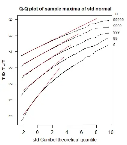
Q-Q plots of maxima of normal samples for n=9, 99, 999, 9999, 99999

In each case, there were 10000 samples generated at a given $n$, yielding 10000 sample maxima for each Q-Q plot.

As you can see for small $n$ like $9$ or $99$, the QQ plot is distinctly curved -- it's not yet well approximated by the Gumbel. But at the largest $n$ here, like $99999$, a Gumbel approximation is quite good; while we can still see a little curvature, it's much more nearly straight.

[The red lines mark in the theoretical line at the values of $a_n$ and $b_n$ given by Alecos at the link. As you see, they have their own issue -- they're essentially the tangent at 0 but that's close to where the curvature looks strongest so they're converging quite slowly to the bulk of the distribution even when it's very close to linear.]

I expect the two effects (the nonlinearity of the plot indicating non-Gumbelness and the fact that the $a_n$ and $b_n$ are far from a line of "best fit" at any given $n$, though they will eventually converge to it) will between them account for the discrepancy you observe.


* It may not be the only issue, but it is definitely an issue. If there are still problems after addressing that, I suggest returning to the divide and conquer approach I was talking about in comments. However, I'd still stick with the suggestion to separate issues with the suitability of the $a_n$ and $b_n$ from those of shape by looking at the Q-Q plot, as well as looking at a sequence of increasingly large $n$.

Glen_b
  • 257,508
  • 32
  • 553
  • 939
  • thanks, there was that and the fact I was not normalizing by quantities $a_n$ and $b_n$ (not even the empirical quantities, see the definition of $f$ I'm throwing into the sampler), but in fact I would have never noticed if I kept the sample size that low. – Vittorio Apicella Sep 21 '19 at 09:53