1

I have two times series: A and B, they are highly correlated. I would like to build the model A~B,however, I have observed that A moves up earlier than B and much faster. Later, after the shock, A decreases also much faster. Do you have any hints how can I build the model?

Files:

a) A: https://1drv.ms/u/s!Am9f1Ox4hcd-6VizdMp9r3sbWIYe?e=HiTGBF

b) B: https://1drv.ms/u/s!Am9f1Ox4hcd-6VkG6TvCkY0Id6DC?e=Fc2OfB

A vs B Hist data

Lohengrin
  • 47
  • 6

2 Answers2

2

I took your 78 quarterly values and arbitrarily selected A as the output series and B as the input. I used AUTOBOX a piece of software that I have helped to develop in it's optionally totally automatic mode. It follows the Transfer Function paradigm http://www.autobox.com/pdfs/A.pdf to form a SARMAX model https://autobox.com/pdfs/SARMAX.pdf .

While both series themselves are non-stationary themselves , the equation/relationship between them required no differencing operators. This phenomenon is not unusual at all .

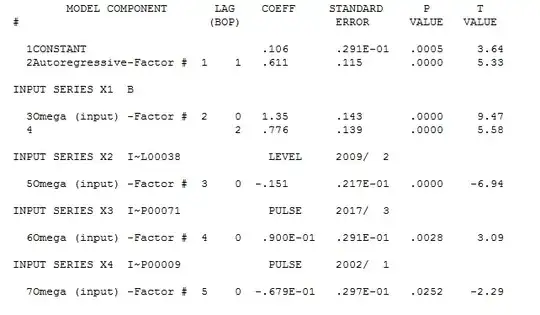
Model diagnostics from a tentative TF model suggested the need for a (visually obvious) level shift indicator at period 38 (2009/2) and two pulse indicators (periods 71 and 9 ... 2017/3 & 2002/1 ) and an AR(1) component.

The model used both a contemporary direct effect of B and an indirect effect of B lagged twice in order to predict Y.

The method used to identify these three latent determinstic structures is here http://docplayer.net/12080848-Outliers-level-shifts-and-variance-changes-in-time-series.html .

The Actual/Fit and Forecast graph is here enter image description here with equation here enter image description here and here enter image description here

The statistics for the model are here enter image description here

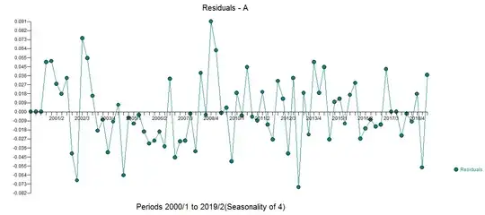
The model residual plot suggests both mean and error variance constancy . enter image description here with an ACF here enter image description here . AUTOBOX at one point tentatively considered a second level shift at period 38 (2009/2) but found it not-significant.

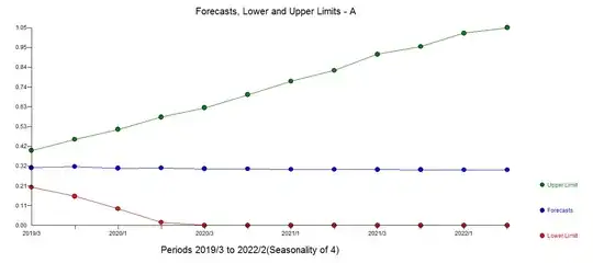
The forecasts for the next 12 quarters reflect the uncertainty in the predictions for the input series B and the possibility of future pulses . enter image description here . The limits were generated using montecarlo procedures providing a complete probability distribution for each forecast period.

The Actuals & Cleansed graph highlight the level shift (intercept change) and the two (now !) clear pulses.

The "shock" that you allude to is a "permanent effect" .

In conclusion to form this model the following 5 characterics needed to be identified

1 What level of differencing needs to be included (if any ) 2 what is the form of the relationship 3 Is there a level shift needed to deal with an exogenous unstated factor 4 are there one-time only effects needed to deal with exogenous factors 5 What is the impact of omitted stochastic series i.e.the form of the ARMA structure. 6 What power transformation or weighted least squares approach is needed to deal with non-constant error variance through time

IrishStat
  • 27,906
  • 5
  • 29
  • 55
  • IrishStat When they give you the data, you know how to treat them! – Fr1 Sep 02 '19 at 01:03
  • 1
    tu ...for your nice words. – IrishStat Sep 02 '19 at 02:25
  • Thank you IrishStat for your work - this is very useful. Could you please help me to understand one of your comment: 'While both series themselves are non-stationary themselves , the equation/relationship between them required no differencing operators. This phenomenon is not unusual at all .' I thought stationarity of the variables is a must? – Lohengrin Sep 06 '19 at 10:46
  • A stationary time series is one whose statistical properties such as mean, variance, autocorrelation, etc. are all constant over time . With causal models the "relationship" between the variables must be the same i.e. constant or stationary or consistent over time . – IrishStat Sep 06 '19 at 11:58
  • iff the model is sufficient then the errors from the model will be information-less being whit noise ..thus predictable. Reversing the equation then leads to predictions which ought to be useful. – IrishStat Sep 06 '19 at 13:54
1

Here is a result in R, using the auto.arima function in the forecast package. auto.arima automatically determines the necessary AR, MA, d, S components and also allows you to include other variables.

> library(readxl)
> A=read_excel("A.xlsx")
> B=read_excel("B.xlsx")

> A1=ts(A$Value,frequency=4)
> B1=ts(B$Value,frequency=4)

> library(forecast)
> mod=auto.arima(A1,xreg=B1,stepwise=F,approximation=F)
> summary(mod)

Series: A1 
Regression with ARIMA(0,1,0) errors 

Coefficients:
        xreg
      0.4091
s.e.  0.1570

sigma^2 estimated as 0.002247:  log likelihood=126.03
AIC=-248.06   AICc=-247.89   BIC=-243.37

Training set error measures:
                       ME       RMSE        MAE        MPE     MAPE
Training set -0.001337502 0.04678851 0.03242543 -0.3753579 5.792672
                  MASE       ACF1
Training set 0.4114466 0.08525872

So the selected model contains only 1 term, the lag of B. Check the residuals:

> checkresiduals(mod)

    Ljung-Box test

data:  Residuals from Regression with ARIMA(0,1,0) errors
Q* = 7.354, df = 7, p-value = 0.393

Model df: 1.   Total lags used: 8

Look OK. Let's try a model without B:

> mod=auto.arima(A1,stepwise=F,approximation=F)
> summary(mod)

Series: A1 
ARIMA(1,1,0) 

Coefficients:
         ar1
      0.1743
s.e.  0.1114

sigma^2 estimated as 0.002369:  log likelihood=123.98
AIC=-243.95   AICc=-243.79   BIC=-239.26

Training set error measures:
                       ME       RMSE        MAE      MPE     MAPE      MASE
Training set -0.001066886 0.04804238 0.03242514 -0.55368 5.841148 0.4114429
                    ACF1
Training set -0.01470753

> checkresiduals(mod)

    Ljung-Box test

data:  Residuals from ARIMA(1,1,0)
Q* = 4.033, df = 7, p-value = 0.776

Model df: 1.   Total lags used: 8

This model is very similar to the previous in terms of accuracy, and includes only 1 AR term, suggesting that you may as well forecast based on A alone.
user2974951
  • 5,700
  • 2
  • 14
  • 27