Why does the mean for a beta distribution when input into the scipy beta cdf not return 0.5?

Question

Very likely I am missing some fundamentals here, or my python coding is not up to scratch.

When I use the standard formula to calculate the mean for a beta distribution ~ $B(\alpha,\beta)$

$$ \mu = \alpha / (\alpha + \beta)$$

Using an $\alpha$ = 0.67 and a $\beta$ = 0.29, I get a $$\mu = 0.69792$$

However, say I use scipy.stats.beta to view the cdf at $\mu$:

I would expect the resultant value to be 0.5

import scipy.stats as stats
alpha = 0.67
beta = 0.29
stats.beta(alpha, beta).cdf(0.69792)

out[1]: 0.3873254007616228

My logic being if I input $\mu$ for a standard normal distribution's cdf I get the below, 0.5 as expected.

stats.norm().cdf(0)

out[1]: 0.5

What am I missing here ?

There's no particular reason why the CDF at $\mu$ would equal 0.5 in this case. It will for symmetric distributions (that have a mean) such as the Normal and for special cases of asymmetric distributions, but the mean is not necessarily equal to the median, so... — jbowman, Aug 05 '19 at 14:57
Ah okay that makes sense, as if I put alpha & beta = 2, I get my expected behavior, however this makes the beta dist. symmetrical — RK1, Aug 05 '19 at 15:00
@RK1 It sounds like you understand what is happening here well enough to answer your own question. — Sycorax, Aug 05 '19 at 15:39
I think I just needed someone to point out the obvious, I was getting pretty confused with all my permutations of alpha & beta — RK1, Aug 05 '19 at 15:48
@Glen_b Indeed, I believe the duplicate can be found in this answer that you wrote! — Sycorax, Aug 06 '19 at 14:54
@Sycorax Thanks. That's pretty close to what I was sort of remembering and it looks like a good duplicate to me. I'd thought there was one like it that actually had beta distributions in it. This one will do quite well. — Glen_b, Aug 06 '19 at 16:03

BruceET · Accepted Answer · 2019-08-06T08:09:56.447

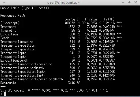
You already have an answer in @jbowman's Comment, but here is some related R code, which I hope you can translate to Python--for the parts of interest.

According to Wikipedia, the approximate median of $\mathsf{Beta}(.67,.29)$ is $\eta = \frac{\alpha - 1/3}{\alpha+\beta-2/3},$ for $\alpha,\beta > 1.$ But that doesn't work for your beta distribution which has population median $\eta = 0.8433177.$ [Improperly applied here, the approximation gives a nonsense value outside the unit interval.]

al = .67;  be = .29;  aprx.med = (al-1/3)/(al+be-2/3);  aprx.med
[1] 1.147727      # (improper) formula
qbeta(.5, al, be)
[1] 0.8433177     # exact median

curve(dbeta(x, al, be), 0, 1, lwd=2, ylab="Density", 
      xlab="x", ylim=c(0,6), main="Density Curve of BETA(.67,.29)")
   abline(v = 0:1, col="green2"); abline(h=0, col="green2")

A sample of size $n = 10^6$ has sample median about 0.8437. [One can show that the 95% margin of error, using the sample median to estimate the population median is about $\pm 1/\sqrt{n} = 0.001.]$

set.seed(1234);  x = rbeta(10^6, al, be)
median(x)
[1] 0.8437234

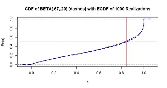
The position of the population median is marked by the vertical line in the following plot of the beta CDF and the empirical CDF (ECDF) of the first thousand points in the sample above. [The ECDF makes a jump of $1/n$ at each (sorted) value of the relevant sample. At the resolution of the figure below, the ECDF appears to be a smooth curve.]

lbl = "CDF of BETA(.67,.29) [dashes] with ECDF of 1000 Realizations"
plot(ecdf(x[1:1000]), main=lbl)
  curve(pbeta(x, al, be), add=T, lwd=3, lty="dashed", col="blue", n=10001)
  abline(v=qbeta(.5,al,be), col="red");  abline(h=.5, col="red")

The exact mean $\mu = \frac{\alpha}{\alpha+\beta} = 0.6979,$ estimated by the sample mean of a sample of a million as $\bar X = \hat \mu = 0.6982 \pm 9.00066.$

al/(al+be)
[1] 0.6979167
mean(x) 
[1] 0.6982305
2*sd(x)/sqrt(10^6)
[1] 0.0006560175    # 95% margin of sim error

Thanks @BruceET, in hindsight when you visualize the CDF it becomes clear, will keep that in mind for next time :) — RK1, Aug 06 '19 at 08:20

Why does the mean for a beta distribution when input into the scipy beta cdf not return 0.5?

1 Answers1