Proportions: why changing to population mean estimator doesn't change the distribution

Question

I saw in a few places (e.g. here) when you compare proportions of 2 samples, under a null hypothesis that they are equal, you eventually get to this:

$$ \frac{\bar X - \bar Y}{\sqrt{P(1-P)(\frac{1}{n} + \frac{1}{m})}} \sim N(0,1) $$

At which point there's a mental "jump" where you estimate $P$ from the total of two samples, and stick it in the above formula, i.e.:

$$ \hat P = \frac{\sum x_i + \sum y_i}{n + m} \\ \frac{\bar X - \bar Y}{\sqrt{\hat P(1- \hat P)(\frac{1}{n} + \frac{1}{m})}} \sim N(0,1) $$

My question is why is it legal to simply stick $\hat P$ instead of $P$ and still assume that it distributes on the standard normal distribution. Is there any proof of this?

UPDATE:

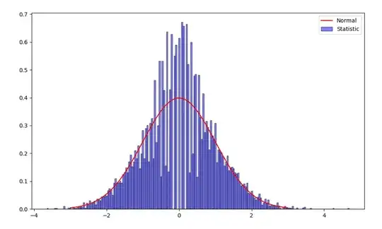
So I tried to simulate it myself, and indeed, when $n \neq m$, the histogram of the proportion statistic looks to fit very well the standard normal distribution.

However, if $n = m$, there seems to be a gap opening in the middle of the distribution:

Code (in Python):

import numpy as np
from scipy import sqrt, stats
from matplotlib import pyplot as plt

# Statistic
p = 0.2
n = 700
m = 300
X = np.random.binomial(n, p, 10000)
Y = np.random.binomial(m, p, 10000)
x_bar = (1/n) * X
y_bar = (1/m) * Y
est_p = (1/(n+m)) * (X + Y)
var = est_p * (1 - est_p) * (1/n + 1/m)
statistic = (x_bar - y_bar)/(sqrt(var))
plt.hist(statistic, density=1, color='blue', edgecolor='black', bins=200, alpha=0.5, label='Statistic')

# Normal
mu = 0
variance = 1
sigma = sqrt(variance)
x = np.linspace(mu - 3*sigma, mu + 3*sigma, 100)
plt.plot(x, stats.norm.pdf(x, mu, sigma), color='red', label='Normal')

plt.legend(loc='upper right')
plt.show()

Answer 1

The substitution of $\hat p$ for $p$ is 'legal' only in the sense that it is a reasonable approximation in some circumstances. The sample sizes $n_1$ and $n_2$ have to be large enough for normal approximations to be valid.

Suppose $X \sim \mathsf{Binom}(n_1, \theta_1),$ $Y \sim \mathsf{Binom}(n_2, \theta_2),$ and we want to use binomial counts $X$ and $Y$ to test $H_0: \theta_1 = \theta_2$ against $H_a: \theta_1 \ne \theta_2.$ Then we use $\hat p_1 = X/n_1$ to estimate $\theta_1$ and $\hat p_2 = Y/n_1$ to estimate $\theta_2.$ And, under $H_0,$ we use $\hat p = (X+Y)/(n_1 + n_2)$ to estimate $\theta = \theta_1 = \theta_2.$

If sample sizes are sufficiently large, then $Z = \frac{\hat p_1 - \hat p_2}{\widehat{SE}} \sim \mathsf{Norm}(0,1),$ where $SE = \sqrt{\theta(1-\theta)(1/n_1 + 1/n_2)},$ and $SE$ is estimated by $\widehat{SE} = \sqrt{\hat p(1-\hat p)(1/n_1 + 1/n_2)}.$

In your example from the link we have $n_1 \approx 300$ and $n_2 \approx 200$ The following simulation shows that those sample sizes are suitable for a normal approximation of the null distribution for $H_0: \theta_1 = \theta_2,$ at least in the 'tail', where judgments to accept or reject are made.

set.seed(731)
th1 = .6; n1 = 300; x=rbinom(10^5, n1, th1)
th2 = .6; n2 = 200; y=rbinom(10^5, n2, th2)
p1 = x/n1;  p2 = y/n2;  p = (x+y)/(n1+n2)
d = p1-p2;  se = sqrt(p*(1-p)*(1/n1 + 1/n2));  z = d/se
hist(z, prob=T, br=40, col="skyblue2")
  curve(dnorm(x), add=T, lwd=2)
  abline(v =c(-1.96,1.96), col="red", lty="dotted")
mean(abs(z) > 1.96)
[1] 0.05046

In the simulations, the z-statistic leads to a test at very nearly the 5% level. The distribution of $Z$ is discrete, slightly smoothed out in the histogram, but still approximately normal in the tails.

By contrast, if sample sizes are $n_1 = 20, n_2 = 15,$ then the simulated distribution of the z-statistic is a poor approximation to normal. The simulated distribution is essentially correct, but it is not clear that that the standard normal distribution leads to a valid test. [The R code for this simulation is omitted because there are only a few changes in code from the previous one.]

The simulated distribution of $Z$ is discrete. Simulated probabilities of its 204 values are plotted below.

Most 'rules of thumb', recommending adequate sample sizes for such tests, are based on simulations.