Let me show some established terminology and notation to try to clarify
what you are doing. There is nothing below that can't be found in a basic
statistics textbook, but I have chosen what to say, hoping specifically
to clear up---in the most compact feasible way--some of the confusion in your question.
Population parameters and estimates from a sample. If $X_1, X_2, \dots, X_m$ is a random sample of size $m$ from a Population A
with distribution $\mathsf{Norm}(\mu_A, \sigma_a),$ then the population mean $\mu_A$ is estimated
by the sample mean $\bar X = \frac 1m \sum_{i=1}^m X_i = \hat \mu_A.$
Also, the population variance
$\sigma_A^2$ is estimated by the sample variance $S_X^2 = \frac{1}{m-1}\sum_{i=1}^m (X_i - \bar X)^2 = \widehat{\sigma_A^2}.$
If the population variance $\sigma_A^2$ is known, then
$$Z_A = \frac{\bar X_A - \mu_A}{\sigma_A/\sqrt{m}} \sim \mathsf{Norm}(0,1),$$
the standard normal distribution.
One-sample tests. If the population variance $\sigma_A^2$ is not known and is estimated by $S_X^2,$ then
$$T_A = \frac{\bar X_A - \mu_A}{S_X/\sqrt{m}} \sim \mathsf{T}(\nu=m-1),$$
Student's t distribution with $m - 1$ degrees of freedom. If $m$ is very large, so that $S_X^2$ estimates $\sigma_A^2$ very closely, then the distribution
$\mathsf{T}(\nu=m-1)$ is very closely approximated by $\mathsf{Norm}(0,1).$
The statistic $T_A$ can be used for one-sample tests and to make confidence intervals for $\mu_A,$ but your Question is about two-sample tests, so I will move on to that.
Similar notation and results hold for a random sample $Y_1, Y_2, \dots Y_n$
from Population B distributed as $\mathsf{Norm}(\mu_B, \sigma_B)$ and for
$Z_B \sim \mathsf{Norm}(0,1)$ and $T_B \sim \mathsf{T}(\nu=n-1).$
Two-sample tests. Now, if you have samples from both populations and you want to test the
null hypothesis $H_0: \mu_A = \mu_B$ against the alternative $H_1: \mu_A \ne \mu_B,$ then the test statistic for a pooled two-sample (or A/B) test is
$$T = \frac{\bar X - \bar Y}{S_p\sqrt{\frac 1m + \frac 1n}} \sim \mathsf{T}(\nu = m+n-2),$$
where $S_p^2 = \frac{(m-1)S_X^2 + (n-1)S_Y^2}{m+m-2}.$ One would reject $H_0$ at the 5% level of significance, if $|T| \ge t_c,$ where $t_c$ cuts probability $0.05/2 = 0.025$ from the upper tail of the distribution $\mathsf{T}(\nu = m+n-2).$
This test is performed under the assumption that the two populations have
the same variance: $\sigma_A^2 = \sigma_B^2 = \sigma^2.$ The 'pooled variance estimate' $S_p^2$ shown above uses information from both samples to estimate
the common population variance $\sigma^2.$
If $m + n$ is very large, so that $S_p^2$ is nearly equal to $\sigma^2,$ then $T$ has nearly a standard normal distribution, so one might reject the null hypothesis if $|T| \ge 1.96.$
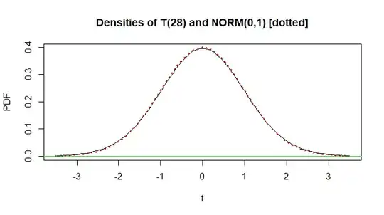
Notes: (1) Some elementary texts say that for testing at the 5% level of significance, 'very large' means something like $m + n > 30.$ One argument is that for 28 degrees of freedom the 5% critical value is $t_c = 2.048,$ which rounds to $2.0,$ as does $1.96.$ Another is that, on a graph as below, it can be difficult to distinguish the density functions of $\mathsf{T}(28)$ (black) and standard normal (dotted red). However, by more precise computation, as @Glen_b comments, that approximation could actually mean testing at about the 6% level.
(2) Unequal variances. If we are unable to assume that $\sigma_A^2 = \sigma_B^2,$ then the
exact test statistic $T$ given above is incorrect and it is difficult to
find the exact distribution of $T.$ However, the Welch two-sample t test
uses a slightly different form of $T$ and a sufficiently accurate approximate
t distribution for most practical applications. Almost all of what I have shown you above still applies, but there is a little more to say. If you are interested in that, perhaps you can find a useful explanation in a statistics text or google 'Welch t test'.
(3) Non-normal data. If data are not normal, then you can hope sample sizes are large enough that sample means are nearly normal and that sample variances closely approximate population variances. Then the two sample $T$-statistic may be nearly normal. This may be useful if population distributions are not markedly skewed. You might search on this site and elsewhere for 'robustness of t tests against non-normal data'.
Addendum: Numerical example. Here is output for a pooled t test from R statistical
software. $n = 12, m = 13,$ $X$'s from $\mathsf{Norm}(\mu_A=100,\sigma=10),$ $Y$'s from $\mathsf{Norm}(\mu_B=112, \sigma=10).$
Because this is a simulation, we know that the population means differ by $12,$ so we can hope the test detects this difference. Because $|T| = 2.28 > t_c = 2.07$ the null hypothesis is indeed rejected.
set.seed(708)   # for reproducibility
x = rnorm(12, 100, 10);  y = rnorm(13, 112, 10)
mean(x);  var(x)
[1] 102.466
[1] 65.76268
mean(y);  var(y)
[1] 111.3025
[1] 119.215
boxplot(x, y, horizontal=T, col="skyblue2", pch=19)
  points(c(mean(x), mean(y)), 1:2, col="red")  $ red circles show means
t.test(x, y, var.eq=T)

        Two Sample t-test

data:  x and y
t = -2.2809, df = 23, p-value = 0.03214
alternative hypothesis:
  true difference in means is not equal to 0
95 percent confidence interval:
 -16.8505188  -0.8224146
sample estimates:
mean of x mean of y
 102.4660  111.3025

c.t = qt(.975, 23);  c.t
[1] 2.068658

