2

I wish to to some simple hypothesis testing of the form provided by T-Tests and ANOVA. However, my data is not normally distributed (it follows a Pareto distribution).

My understanding is that T-Tests make the assumption that the data is normally distributed and hence I won't be able to use them - is that correct? Is there something else I can do?

EDIT Here is some more info about my problem.

I'm trying to do some quality analysis on software defects, and am having trouble knowing where to start. One basic question I want to answer is:

Does software produced in department X have more defects than department Y?

As some background, we group changes to software as "patches", in which case the question becomes

Does the average patch from department X have more defects than department Y?

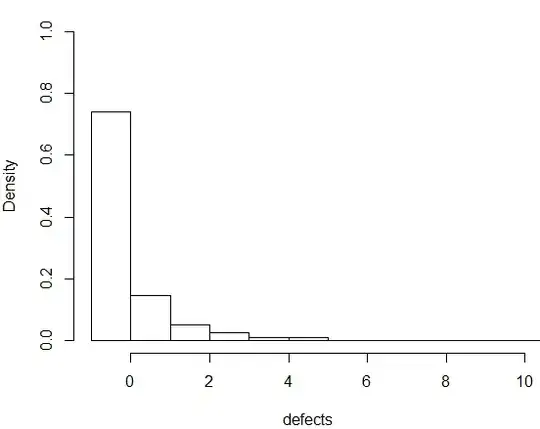
Here is a histogram of bugs / patch, N = 3700.

bugs/patch

There is a philosophical issue of what it means to have "more" defects that I don't have a great answer to. The obvious choice for one of my limited knowledge is to compare the mean defects in each group, but as others have pointed out that's not clearly the best choice. The measure linked to by Procrastinator ($P(X<Y)$) seems like it captures my intuition well.

Xodarap
  • 2,448
  • 2
  • 17
  • 24
  • Thanks @Procrastinator! My goal is to analyze whether certain business processes lead to a decrease in defects. Defects are in general Pareto-distributed (almost all instances cause zero defects, but a few cause many), and I wish to answer questions like "does department X cause more defects than department Y?" – Xodarap Oct 30 '12 at 17:09
  • 1
    Then [this question](http://stats.stackexchange.com/q/30141/10525) and the answers there might be of interest. –  Oct 30 '12 at 17:11
  • It may just be my ignorance, but I thought Pareto variates were continuous and strictly positive... how did you determine that the Pareto was a reasonable fit to your data? – jbowman Oct 30 '12 at 19:25
  • @jbowman: Incorrectly, perhaps. I basically looked at a QQ-plot - you're right that since my data has $P(X = 0) > 0$ it's not really Pareto, but I'm not sure what the correct term is. Perhaps I should say it obeys some power law distribution? – Xodarap Oct 30 '12 at 19:39
  • @Xodarap In the light of this new information, you should consider using a mixture of a discrete and a continuous distribution for modelling these data. However, if you could provide more information about your data and possibly a histogram, that would help us to avoid type III error. –  Oct 30 '12 at 20:32
  • 1
    @Procrastinator: I have updated the question. – Xodarap Oct 30 '12 at 21:20
  • So, are the data discrete? –  Oct 31 '12 at 13:40
  • Yes, it is impossible to cause a non-integer number of defects. However, we could imagine controlling for patch size as e.g. defects / lines of code, at which point it would be continuous (note that there would still be a bump at "0" since the numerator would be zero). I'd be thankful for help in either direction. – Xodarap Oct 31 '12 at 14:41
  • So 1) find best-fit Lomax distribution (it looks like there are R packages for this) then 2) find $P(X – Xodarap Oct 31 '12 at 20:16
  • 2
    @Xodarap I have been thinking a bit about this problem. It seems like you need a distribution that can account for $P(X=0)\gt 0$ and takes values in $(0,\infty)$ as well. For this, you need a mixture of a discrete and a continuous distribution. I have not figured out how to estimate $P(X –  Nov 01 '12 at 14:35
  • I'm wondering if dividing it into 0 vs. non-zero would be a better idea. Then I could model it as a weighted coin, which I think is less confusing. What do you think? – Xodarap Nov 01 '12 at 22:11
  • @Xodarap I do not see a reason for doing so. Separating these observations implies that they come from different populations (which is not the case, I think). How many observations you have? What I would do is to 1) calculate the Mann-Whitney estimator; 2) Bootstrap: resample with replacement, say 1000 times, and recalculate this estimator; 3) Calculate a confidence interval using this sample of estimators. Use this confidence interval to draw conclusions about the departments. For example, if a 95% confidence interval does not include the value $0.5$, then there is evidence of a difference. –  Nov 02 '12 at 10:30
  • 1
    Procrastinator: My worry is that I can separate bad from really bad. However, I can't separate good from really good (they both have 0 defects). If I made it dichotomous I would remove this inconsistency. My N=3700, I will try your method with some sanity checks and see what happens, thanks! – Xodarap Nov 02 '12 at 14:08

1 Answers1

2

Interesting problem. This looks like an independent probability problem rather than a statistics problem, i.e., not a problem yielding a statistic like a $t$-statistic. For example, if the probability of having zero defects is 80%, then the probability of having one or more defects is 20%. If we assume that the probability of having any defect is unrelated to whether or not there is a defect in the "object" already, then yes, the probabilities chain, and look like a power function, because it is a power function. This relates to the probability of having only one defect ($p$) as $\sum _{i=1}^{\infty } p^i=\frac{p}{1-p}$. So for our example, we ask how did we get to having a 20% total defect rate and the answer is when single failure rate is $\frac{p}{1-p}=0.2$ or $p=\frac{1}{6}$.

Now the second part of the question is when is a failure rate significantly different from another failure rate. I think that this means that once we have the single failure rate from one experiment, $p1$, and another single failure rate from another experiment, $p2$, we can do a two-sample binomial probability test as outlined here. That is, I think so, but, we may need to be careful with what numbers we are substituting in. For example, the total number I do not think includes the multiple failure objects, just the number with no failures and those with single failures for the two-sample test. So now comes the tricky part, the calculated single failure rate from including multiple failures as part of the calculation may differ from the observed number of objects with only a single failure. It may be better to use the calculated single failure rate, rather than the observed rate, and it is even possible to calculate binomial probabilities for non-integer numbers of observations by using a continuous form of the binomial distribution. However, for approximate answers and for a large number of observations, that may be overkill, and nearest integer results are likely good enough for most purposes.

Carl
  • 11,532
  • 7
  • 45
  • 102