The variance of the derivative of a Gaussian process, $f$, is given by (9.1):
$$ Var(\frac{\partial f}{\partial x}) =\frac {\partial ^2 k(x,x)}{\partial x^2},$$
where $k(·, ·)$ is both a positive-definite quantity and the covariance function of $f$. But when evaluating the error corresponding to $\frac{\partial f}{\partial x}$, we observe that it is instead given by $\frac {\partial ^2 k(x,x)}{\partial x^2}$, which is not necessarily positive everywhere. Therefore is the above definition for $Var(\frac{\partial f}{\partial x})$ actually correct? Is it valid to simply take the absolute value of this quantity when computing the error or should this variance be handled differently?
Example:
import numpy as np
from matplotlib import pyplot as plt
from sklearn.gaussian_process import GaussianProcessRegressor
from sklearn.gaussian_process.kernels import RBF, ConstantKernel as C

def f(x):
    """The function to predict."""
    return 1.5*(1. - np.tanh(100.*(x-0.96))) + 1.5*x*(x-0.95) + 0.4 + 1.5*(1.-x)* np.random.random(x.shape)

# Instantiate a Gaussian Process model
kernel = C(10.0, (1e-5, 1e5)) * RBF(10.0, (1e-5, 1e5))

X = np.array([0.803,0.827,0.861,0.875,0.892,0.905,
                0.91,0.92,0.925,0.935,0.941,0.947,0.96,
                0.974,0.985,0.995,1.0])
X = np.atleast_2d(X).T

# Observations and noise
y = f(X).ravel()
noise = np.linspace(0.4,0.3,len(X))
y += noise

# Instantiate a Gaussian Process model
gp = GaussianProcessRegressor(kernel=kernel, alpha=noise ** 2,
                              n_restarts_optimizer=10)
# Fit to data using Maximum Likelihood Estimation of the parameters
gp.fit(X, y)

# Make the prediction on the meshed x-axis (ask for MSE as well)
x = np.atleast_2d(np.linspace(0.8, 1.02, 1000)).T
y_pred, sigma = gp.predict(x, return_std=True)

plt.figure()
plt.errorbar(X.ravel(), y, noise, fmt='k.', markersize=10, label=u'Observations')
plt.plot(x, y_pred, 'k-', label=u'Prediction')
plt.fill(np.concatenate([x, x[::-1]]),
         np.concatenate([y_pred - 1.9600 * sigma,
                        (y_pred + 1.9600 * sigma)[::-1]]),
         alpha=.1, fc='k', ec='None', label='95% confidence interval')
plt.xlabel('x')
plt.ylabel('y')
plt.xlim(0.8, 1.02)
plt.ylim(0, 5)
plt.legend(loc='lower left')
plt.show()

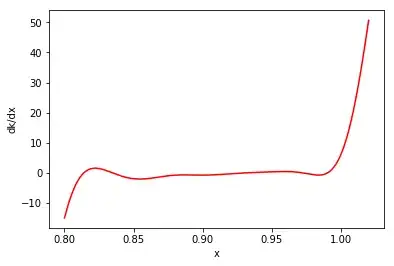
dkdx = np.gradient(sigma**2.,x[:,0])
d2kdx2 = np.gradient(dkdx,x[:,0])

plt.figure()
plt.plot(x, sigma**2., 'k-')
plt.ylabel('k')
plt.xlabel('x')
plt.show()

plt.figure()
plt.plot(x, dkdx, 'r-')
plt.ylabel('dk/dx')
plt.xlabel('x')
plt.show()

plt.figure()
plt.plot(x, d2kdx2, 'g-')
plt.ylabel('d2k/dx2')
plt.xlabel('x')
plt.show()
As a simple analytic case, if we consider a modified squared exponential kernel centered at $x_a$ and $x_b$, then $k(x_i,x_j) = \exp(-(x_i-x_a)^2 - (x_j-x_b)^2)$. This is positive definite. But $\frac {\partial k(x_i,x_j)}{\partial x_i} = -2(x_i - x_a) k(x_i, x_j)$ and $\frac {\partial k(x_i,x_j)}{\partial x_i \partial x_j} = 4(x_i - x_a)(x_j - x_b) k(x_i, x_j)$, which can both possibly be negative.
As you may note, it appears $k$ is always greater than zero, but ${\partial ^2 k(x,x)}/{\partial x^2}$ and ${\partial k(x,x)}/{\partial x}$ can still be negative.


