sklearn Support Vector Regression - test data prediction is constant

Question

I am just getting into learning some basic machine learning for a project at university and I am having a little trouble with SVR on sklearn.

When training a model I can change the epsilon value and see the prediction changing from almost perfect replication to good estimates. However nothing I seem to do changes the output predictions on the testing data, the values are constant. I have a feeling it could be due to data formatting because at one point I changed the index column to be the first column on my csv and the first testing output changed however after that they became constant again.

import numpy as np
import pandas as pd

KPN = pd.read_csv('Regression.csv').astype('float32')

def Split_Train_Test(data, test_ratio):
    train_set_size = 1 - int(len(data) * test_ratio)
    train_set = data[:train_set_size]
    test_set = data[train_set_size:]
    return train_set, test_set

train, test = Split_Train_Test(KPN, 0.1)

The data has 1200 rows so I am just going to use the first 100 for an example:

X = train.iloc[:50,0:1]
y = train["output"][0:50]
X_test = train.iloc[50:100,0:1]


from sklearn.svm import SVR
svr_rbf = SVR(kernel='rbf', epsilon=0.05)
svr_rbf.fit(X,y)

svr_rbf.predict(X)
array([2.72315689, 2.65343986, 2.61527852, 2.63005085,...,2.53509259])

svr_rbf.predict(X_test)
array([2.5851449, 2.6134029 , 2.6134029, 2.6134029,..., 2.6134029])

The X values are just time points, so 1,2,3,.... and the Y values are just points of a time series.

edit: Added time plots

Answer 1

What is observed is a direct consequence of using a potentially improper parameter set for svr. It appears that especially the epsilon used, i.e. the minimum distance between actual and predicted values that needs to be observed so a penalty is induced during fitting, is somewhat large; therefore errors are not adequately penalised and this leads to potential under-fitting. In addition as there is an obvious sequential nature to our data, the influence of the parameter gamma, i.e. how far the influence of a single training example reaches, is going to be important too.

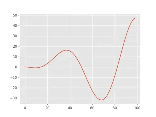
I quickly eye-balled the data from the graph shown and made some quick predictions to show how strong the effect of epsilon can be in this case.

Some final application-specific comments:

1. The flat estimate is not necessarily bad! Off the bat I would say it is actually "correct"; following Makrydakis et al. (2018) Statistical and Machine Learning forecasting methods: Concerns and ways forward setting epsilon "equal to the noise level of the training sample" is a perfectly reasonable thing to start with. "Beating the historical mean" as a forecast (as the current flat-line suggests), is not as trivial as it sounds (see the excellent CV thread on : Is it unusual for the MEAN to outperform ARIMA? for more details).
2. Time-series forecasting tasks tend to be dominated by exponential smoothing and/or ARIMA models; SVMs, while promising, never really established themselves as a strong alternative. I would suggest you consider such approaches if you have not done already.
3. Consider using rolling time-window approach when cross-validating the fitting procedure for a time-series model. Rob Hyndman has written extensively on time-series cross-validation, his book with Athanasopoulos has a very nice section about this available here. In Python check TimeSeriesSplit from sklearn.model_selection.

Code:

import numpy as np
import pandas as pd
import matplotlib.pyplot as plt
from sklearn.svm import SVR

dtrain=np.random.uniform(0,0.00100,[100,2])      
dtrain[:50,1] = np.array([2.770, 2.690, 2.560, 2.630, 2.730, 2.720, 2.690, 2.680, 2.600, 2.630, 
                          2.580, 2.615, 2.72,  2.670, 2.690, 2.710, 2.705, 2.660, 2.610, 2.580, 
                          2.650, 2.600, 2.550, 2.600, 2.630, 2.61,  2.620, 2.660, 2.670, 2.665, 
                          2.595, 2.625, 2.685, 2.680, 2.650, 2.660, 2.550, 2.540, 2.520, 2.486, 
                          2.551, 2.551, 2.580, 2.605, 2.525, 2.510, 2.510, 2.480, 2.515, 2.485])
dtrain[:,0] = np.arange(1,101)

X = dtrain[:50,0]
y = dtrain[:50,1]
X_test = dtrain[50:99,0]

svr_rbf_original = SVR(kernel='rbf', epsilon=0.05) 
svr_rbf_original.fit(X.reshape(-1,1),y)
svr_rbf_twicked = SVR(kernel='rbf', epsilon=0.003, gamma=0.001)
svr_rbf_twicked.fit(X.reshape(-1,1),y)

plt.plot(X, y,linestyle="",marker="o", label='Raw')  
plt.plot(X, svr_rbf_original.predict(X.reshape(-1,1)), label='Within sample fit')
plt.plot(X_test, svr_rbf_original.predict(X_test.reshape(-1,1)), label='Fit eps:0.05')
plt.plot(X_test, svr_rbf_twicked.predict(X_test.reshape(-1,1)), label='Fit eps:0.003 / gamma:0.001') 
plt.legend() 
plt.show()