Beta regression - interpret coefficients using loglog link

Question

Although a number of similar questions (some of them duplicates) have been asked around the interpretation of the coefficients from a beta regression, these seem to be focused on models that have used the logit link, but I am yet to find one focused on the log-log link, and I do not know if the interpretation is the same.

I have two questions ...

1.I have posted previously about computing the regression equation from a betareg model when using the log-log link which has been answered, and now I would like to understand how to interpret the coefficients. As stated in my previous question, I am familiar with interpreting the outputs from multiple regression models, which take the following form.

Assuming all other factors are held constant, a one unit increase in x is associated with an increase/decrease in y.

I would like to understand how I take the coefficients from the beta regression output using the log-log link and get to a similar outcome phrase - if such a simple phrase is possible. I have posted the example output below that I used in my previous question.

Call:
betareg(formula = y ~ x1 + x2, link = "loglog")

Standardized weighted residuals 2:
    Min      1Q  Median      3Q     Max 
-1.4901 -0.8370 -0.2718  0.2740  2.6258 

Coefficients (mean model with loglog link):
            Estimate Std. Error z value Pr(>|z|)  
(Intercept)    1.234      1.162   1.062   0.2882  
x1            31.814     26.715   1.191   0.2337  
x2            -7.776      3.276  -2.373   0.0176 *

Phi coefficients (precision model with identity link):
      Estimate Std. Error z value Pr(>|z|)  
(phi)    24.39      10.83   2.252   0.0243 *
---
Signif. codes:  0 '***' 0.001 '**' 0.01 '*' 0.05 '.' 0.1 ' ' 1 

Type of estimator: ML (maximum likelihood)
Log-likelihood: 12.06 on 4 Df
Pseudo R-squared: 0.2956
Number of iterations: 232 (BFGS) + 12 (Fisher scoring) 

2. In multiple regression, it is possible to understand the influence of each coefficient on the model, by considering the size of the standardised coefficient. Is it possible to get a similar insight based on the outcome of the beta regression?

I would appreciate any advice.

Answer 1

The interpretation with the log-log link function is not the same, and, indeed there is no easy way to use it to really interpret the effect like you do for linear regression or with other link functions in generalized linear models. To be sure, assume, WLOG that you are interested in studying a $c$-unit increase in the predictor $X_1$. Then under the original link function, before any increase you would have:

\begin{eqnarray*} -\log(\log(p)) & = & X^{\top}\boldsymbol{\beta} \end{eqnarray*}

and after a $c$-unit increase in $X_1$ you have:

\begin{equation} \begin{alignedat}{2} \Rightarrow\quad && \ -\log(-\log(p^*)) &= X^{\top}\boldsymbol{\beta}+c\beta_{1} \\ \Rightarrow\quad && -\log(-\log(p^*)) &= -\log(-\log(p))+c\beta_{1} \\ \Rightarrow\quad && \log(-\log(p))-\log(-\log(p^*)) &= c\beta_{1} \\ \Rightarrow\quad && \log\left(\frac{-\log(p)}{-\log(p^*)}\right) &= c\beta_{1} \\ \Rightarrow\quad && \frac{\log(p)}{\log(p^*)} &= e^{c\beta_{1}} \\ && \end{alignedat} \end{equation}

By examining the last terms, you see there really doesn't appear to be a nice way to describe, in words, a $c$-unit increase in a predictor at least in any comprehensible way.

This is generally why, for example, folks like Hosmer, Lemeshow, and Sturdivant, recommend using specific link functions when attempting to interpret parameters and different link functions all together when the primary goal is to calculate estimates of the proportion. They write:

"If the goal of the analysis is to obtain estimates of the probability (proportion) of the outcome and estimates of effect for individual model covariates are, at best, of secondary importance, then we recommend that one consider the Probit, complementary log-log or log-log link models... If the goal of the analysis is to provide an alternative to the odds ratio as a measure of the effects of model covariates then we recommend using either the log link or identity link" (p. 436).

Answer 2

As discussed by @StatsStudent and in the comments: There is no simple and intuitive ceteris paribus interpretation for log-log links. The easiest link that still assures predictions are in $(0, 1)$ is the logit link, see: interpretation of betareg coef However, even in that case it takes some practice to quickly process the meaning of coefficients.

Hence, in general I recommend to complement other analyses by looking at predictions and discrete changes for regressor combinations of interest. I typically set up some new dummy data set that contains combinations of regressor values that I'm interest in and then I look at predictions, e.g., of means, variances, medians, or other quantiles.

As a simple example, consider your artificial data:

d <- data.frame(
  x1 = c(0.051, 0.049, 0.046, 0.042, 0.042, 0.041, 0.038, 0.037, 0.043, 0.031),
  x2 = c(0.11, 0.12, 0.09, 0.21, 0.18, 0.11, 0.13, 0.11, 0.08, 0.10),
  y  = c(0.97, 0.87, 0.77, 0.65, 0.77, 0.84, 0.76, 0.73, 0.82, 0.90)
)
m <- betareg(y ~ x1 + x2, data = d, link = "loglog")

Then, we create a new dummy data set that fixed x1 at its mean and lets x2 vary across its range:

nd <- data.frame(x1 = 0.042, x2 = 8:21/100)

To this data set we can then add the predicted means which show what a 0.01 unit change in x2 does:

nd$mean <- predict(m, nd, type = "response")
nd
##       x1   x2      mean
## 1  0.042 0.08 0.8671101
## 2  0.042 0.09 0.8571699
## 3  0.042 0.10 0.8465540
## 4  0.042 0.11 0.8352276
## 5  0.042 0.12 0.8231556
## 6  0.042 0.13 0.8103037
## 7  0.042 0.14 0.7966381
## 8  0.042 0.15 0.7821265
## 9  0.042 0.16 0.7667387
## 10 0.042 0.17 0.7504468
## 11 0.042 0.18 0.7332267
## 12 0.042 0.19 0.7150583
## 13 0.042 0.20 0.6959266
## 14 0.042 0.21 0.6758232

Clearly the effect of a 0.01 unit change in x2 leads to different predicted changes in the expectation of y:

summary(diff(nd$mean))
##     Min.  1st Qu.   Median     Mean  3rd Qu.     Max. 
## -0.02010 -0.01722 -0.01451 -0.01471 -0.01207 -0.00994 

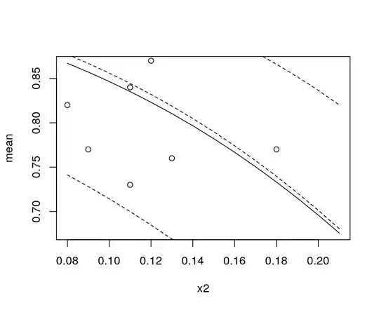
The changes can also be brought out graphically. The code below shows the mean (solid) along with the corresponding 5%, 50%, and 95% quantile (dashed) of the predicted beta distribution. Also, the observations from d are added:

plot(mean ~ x2, data = nd, type = "l")
lines(nd$x2, predict(m, nd, type = "quantile", at = 0.5), lty = 2)
lines(nd$x2, predict(m, nd, type = "quantile", at = 0.05), lty = 2)
lines(nd$x2, predict(m, nd, type = "quantile", at = 0.95), lty = 2)
points(y ~ x2, data = d)

Note, however, that in the actual data d the variable x1 varies along with x2 while in the new dummy data nd the variable x1 is fixed. More generally plotting something like partial residuals would be better than actual observations.

A more formal way of looking at such "effects" displays is provided in packages effects (see http://doi.org/10.18637/jss.v087.i09 and the earlier references therein) or lsmeans (see https://doi.org/10.18637/jss.v069.i01).