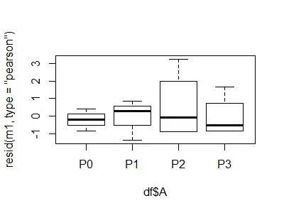
I fitted a beta regression on some proportion data using the betareg() function from the betareg package. The proportion was scaled using the ad-hoc scaling procedure recommended in the betareg vignette (Section 2; 1st paragraph):
vignette("betareg", package = "betareg")
My sample size is $n = 4$, which I know is very limited. After plotting the residuals I saw evidence of heteroskedasticity and decided to include the precision parameter $\phi$ into the model. After that the residuals looked fine and I wanted to get the estimated marginal means of the model using the emmeans() function from the emmeans package. There I saw that one of the lower confidence limits extends into the negative (only for the model that includes $\phi$ though).
My question is, is that possible given the beta distribution?
Below a reproducible example:
df <- structure(list(A = structure(c(1L, 1L, 1L, 1L, 2L, 2L, 2L, 2L,
3L, 3L, 3L, 3L, 4L, 4L, 4L, 4L), .Label = c("P0", "P1", "P2",
"P3"), class = "factor"), PROP = c(0.2, 0.1, 0.2, 0.3, 0.1, 0.4,
0.4, 0.5, 0.5, 0, 0, 0.2, 0.2, 0.5, 0.1, 0.1), PROP_SCALED = c(0.2046875,
0.10625, 0.2046875, 0.303125, 0.10625, 0.4015625, 0.4015625,
0.5, 0.5, 0.0078125, 0.0078125, 0.2046875, 0.2046875, 0.5, 0.10625,
0.10625)), class = "data.frame", row.names = c(NA, -16L))

require(betareg)
require(emmeans)

m1 <- betareg(PROP_SCALED ~ A, data = df)
# summary(m1)
plot(resid(m1, type = "pearson") ~ df$A)
m2 <- betareg(PROP_SCALED ~ A | A, data = df)
# summary(m2)
plot(resid(m2, type = "pearson") ~ df$A)
Note the negative LCL for P2:
emmeans(m2, "A")
#A     emmean         SE  df   asymp.LCL asymp.UCL
#P0 0.2044328 0.03557230 Inf  0.13471239 0.2741532
#P1 0.3453680 0.07860826 Inf  0.19129859 0.4994373
#P2 0.1722369 0.09659308 Inf -0.01708209 0.3615558
#P3 0.2335368 0.07133364 Inf  0.09372545 0.3733482

#Confidence level used: 0.95
For comparison the emmeans for the model without $\phi$:
emmeans(m1, "A")
#A     emmean         SE  df  asymp.LCL asymp.UCL
#P0 0.2386583 0.07473188 Inf 0.09218648 0.3851300
#P1 0.3506016 0.08650745 Inf 0.18105014 0.5201531
#P2 0.1157728 0.04966404 Inf 0.01843309 0.2131125
#P3 0.2407182 0.07502464 Inf 0.09367255 0.3877638

#Confidence level used: 0.95

