ROC curve for discrete classifiers like SVM: Why do we still call it a "curve"?, Isn't it just a "point"?

Question

In the discussion : how to generate a roc curve for binary classification, I think that the confusion was that a "binary classifier" (which is any classifier that separates 2 classes) was for Yang what is called a "discrete classifier" (which produces discrete outputs 0/1 like an SVM) and not continuous outputs like ANN or Bayes classifiers ... etc. So, the discussion was about how the ROC is plotted for "binary continuous classifiers", and the answer is that the outputs are sorted by their scores since the outputs are continuous, and a threshold is used to produce each point on the ROC curve.

My question is for "binary discrete classifiers", such as SVM, the output values are 0 or 1. So the ROC produces just one point and not a curve. I'm confused as to why we still call it a curve?!! Can we still talk about thresholds? How can one use thresholds in SVM in particular? How can one compute the AUC?, Does cross-validation play any role here?

Answer 1

• Yes, there are situations where the usual receiver operating curve cannot be obtained and only one point exists.

• SVMs can be set up so that they output class membership probabilities. These would be the usual value for which a threshold would be varied to produce a receiver operating curve.
  Is that what you are looking for?

• Steps in the ROC usually happen with small numbers of test cases rather than having anything to do with discrete variation in the covariate (particularly, you end up with the same points if you choose your discrete thresholds so that for each new point only one sample changes its assignment).

• Continuously varying other (hyper)parameters of the model of course produces sets of specificity/sensitivity pairs that give other curves in the FPR;TPR coordinate system.
  The interpretation of a curve of course depends on what variation did generate the curve.

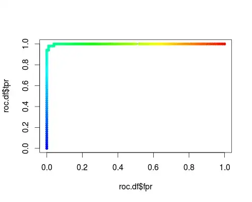
Here's a usual ROC (i.e. requesting probabilities as output) for the "versicolor" class of the iris data set:

• FPR;TPR (γ = 1, C = 1, varying probability threshold):
  

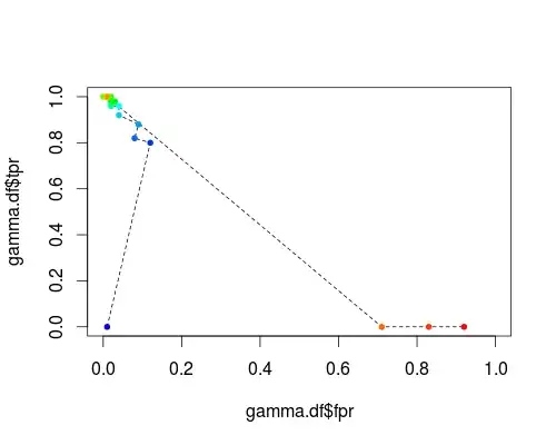
The same type of coordinate system, but TPR and FPR as function of the tuning parameters γ and C:

• FPR;TPR (varying γ, C = 1, probability threshold = 0.5):
  

• FPR;TPR (γ = 1, varying C, probability threshold = 0.5):
  

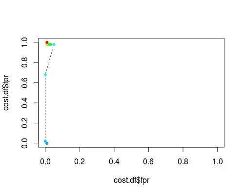
These plots do have a meaning, but the meaning is decidedly different from that of the usual ROC!

Here's the R code I used:

svmperf <- function (cost = 1, gamma = 1) {
    model <- svm (Species ~ ., data = iris, probability=TRUE, 
                  cost = cost, gamma = gamma)
    pred <- predict (model, iris, probability=TRUE, decision.values=TRUE)
    prob.versicolor <- attr (pred, "probabilities")[, "versicolor"]

    roc.pred <- prediction (prob.versicolor, iris$Species == "versicolor")
    perf <- performance (roc.pred, "tpr", "fpr")

    data.frame (fpr = perf@x.values [[1]], tpr = perf@y.values [[1]], 
                threshold = perf@alpha.values [[1]], 
                cost = cost, gamma = gamma)
}

df <- data.frame ()
for (cost in -10:10)
  df <- rbind (df, svmperf (cost = 2^cost))
head (df)
plot (df$fpr, df$tpr)

cost.df <- split (df, df$cost)

cost.df <- sapply (cost.df, function (x) {
    i <- approx (x$threshold, seq (nrow (x)), 0.5, method="constant")$y 
    x [i,]
})

cost.df <- as.data.frame (t (cost.df))
plot (cost.df$fpr, cost.df$tpr, type = "l", xlim = 0:1, ylim = 0:1)
points (cost.df$fpr, cost.df$tpr, pch = 20, 
        col = rev(rainbow(nrow (cost.df),start=0, end=4/6)))

df <- data.frame ()
for (gamma in -10:10)
  df <- rbind (df, svmperf (gamma = 2^gamma))
head (df)
plot (df$fpr, df$tpr)

gamma.df <- split (df, df$gamma)

gamma.df <- sapply (gamma.df, function (x) {
     i <- approx (x$threshold, seq (nrow (x)), 0.5, method="constant")$y
     x [i,]
})

gamma.df <- as.data.frame (t (gamma.df))
plot (gamma.df$fpr, gamma.df$tpr, type = "l", xlim = 0:1, ylim = 0:1, lty = 2)
points (gamma.df$fpr, gamma.df$tpr, pch = 20, 
        col = rev(rainbow(nrow (gamma.df),start=0, end=4/6)))

roc.df <- subset (df, cost == 1 & gamma == 1)
plot (roc.df$fpr, roc.df$tpr, type = "l", xlim = 0:1, ylim = 0:1)
points (roc.df$fpr, roc.df$tpr, pch = 20, 
        col = rev(rainbow(nrow (roc.df),start=0, end=4/6)))

Answer 2

Normally, the predicted label $\hat{y}$ from SVM is given by $\hat{y}=\mbox{sign}({\mathbf w^T x}+b)$, where ${\mathbf w}$ is the SVM-optimized weights of the hyper-plane, and the $b$ is the SVM-optimized intercept. This can also be re-written as follows: \begin{eqnarray} \hat{y} & = & \left\{\begin{array}{cc} 0 & \mbox{if}~~{\mathbf w^T x}+b < 0 \\ 1 & \mbox{otherwise} \end{array} \right. \end{eqnarray}

However, if we introduce a threshold $\eta$, we can control the positive detection rate by varying $\eta$, i.e. \begin{eqnarray} \hat{y} & = & \left\{\begin{array}{cc} 0 & \mbox{if}~~{\mathbf w^T x}+b < \eta \\ 1 & \mbox{otherwise} \end{array} \right. \end{eqnarray}

By varying $\eta$, we can produce an ROC using SVM, and thereby adjusting the sensitivity and specificity rate.

For example, if we want to do it in python, we can extract ${\mathbf w}$ and $b$ using threshold $\eta$ as follows.

>>> from sklearn.svm import SVC
>>> model = SVC(kernel='linear', C=0.001, probability=False, class_weight='balanced')
>>> model.fit(X, y)
>>> # The coefficients w are given by
>>> w = list(model.coef_)
>>> # The intercept b is given by
>>> b = model.intercept_[0]
>>> y_hat = X.apply(lambda s: np.sum(np.array(s)*np.array(w))+b, axis=1)
>>> y_hat = (y_hat > eta).astype(float)

Answer 3

The ROC curve plots specificity vs sensitivity which varies with threshold of a covariate (which may be continuous or discrete). I think you are confusing the covariate with the response and perhaps do not fully understand what an ROC curve is. It is certainly a curve, if the covariate is continuous and we look at a threshold for the covariate changing continuously. If the covariate is discrete you can still plot it as a function of a continuous threshold. Then the curve would be flat with steps up (or down) at thresholds that correspond to the discrete values of the covariate. So this would apply to SVM and any other discrete classifiers.

Regarding AUC since we still have an ROC (an estimated one), we can still compute the area under it. I am not sure what you had in mind with your question about cross-validation. In the context of classification problems, cross-validation is used to get unbiased or nearly unbiased estimates of error rates for the classifier. So it can enter into how we estimate the points on the ROC.