What test to use to find the probability of highest value?

Question

If I have a vector of around 40 values each with a normally distributed error, is there an easy way to figure out the probability of each element being the element with maximal true value? For context, this is coming from an idea to combine a min-max search with monte-carlo-tree search for use in the Leela Chess project.The idea would be to replace the average of nodes used in a plain mcts with a weighted average where the weights are the probability a given move is the best one.

It is probably worth noting that the method I need does not need to be accurate (within 1% should be fine), but needs to be very efficient as it will be run up to 100,000x per second. Bonus points for methods that can be updated on the fly, as that will make it much faster for the application.

Answer 1

This problem gives a formula for the desired probability, but it is a complicated formula involving integration, that requires some kind of numerical evaluation. Let $\mathbf{x} = (x_1,...,x_n) \in \mathbb{R}^n$ be a vector of values and let $\boldsymbol{\varepsilon} = (\varepsilon_1,...,\varepsilon_n) \sim \text{IID N}(0, \sigma^2)$ be a corresponding vector of errors that are added to the values. The maximum of the error-inclusive values is denoted as:

$$M \equiv \max (x_1+\varepsilon_1,...,x_n+\varepsilon_n).$$

Let $\Phi$ and $\phi$ denote the CDF and PDF for the standard normal distribution. The probability that the $k$th element of the error-inclusive values achieves the maximum value can be written as:

$$\begin{equation} \begin{aligned} p_k &\equiv \mathbb{P}(x_k+\varepsilon_k = M) \\[6pt] &= \int \limits_{-\infty}^\infty \mathbb{P}(x_k+\sigma e = M | \varepsilon_k= \sigma e) \phi(e) de \\[6pt] &= \int \limits_{-\infty}^\infty \Big( \prod_{i \neq k} \mathbb{P}(x_i + \varepsilon_i < x_k + \sigma e) \Big) \phi(e) de \\[6pt] &= \int \limits_{-\infty}^\infty \Big( \prod_{i \neq k} \Phi \Big( \frac{x_k-x_i}{\sigma} + e \Big) \Big) \phi(e) de. \\[6pt] \end{aligned} \end{equation}$$

This is a one-dimensional integral using well-known functions (the CDF and PDF of the normal distribution) that are programming into most statistical programming packages. The integral does not have a closed-form solution, so you are going to need to use some kind of numerical method to approximate its value, and that is going to raise computational issues. It is relatively simple to generate an estimate of this integral via importance sampling:

$$p_k \approx \frac{1}{M} \sum_{\ell=1}^M \prod_{i \neq k} \Phi \Big( \frac{x_k-x_i}{\sigma} + e_\ell \Big) \quad \quad \quad e_1,...,e_M \sim \text{IID N}(0,1).$$

As an example, I will show you how to estimate these probabilities in R using the importance sampling approximation. Using ten randomly generated starting points I get probabilities shown in the plot below. (The black points show the ten $x_i$ values and the red bars show their respective probability of being the highest element once we add an error term.

---

R code: This is the R code to create a vectorised function that estimates the probabilities for each element via importance sampling with $W$ iterations, and then norms this probability vector to sum to one. For large $W$ this should give you a reasonable approximation to the true probabilities. This code includes the function and the plot code:

#Create vectorised function to estimate probabilities
ESTIMATE_PROBS <- function(x, sigma = 1, W = 10^6) {
    EEE   <- rnorm(W,0,1);
    K     <- length(x);
    PROBS <- rep(0,K);
    for (k in 1:k) { 
        PPP <- rep(0,W);
        for (w in 1:W) { PPP[w] <- prod(pnorm((x[k]-x[-k])/sigma + EEE[w], 0, 1)); }
        PROBS[k] <- mean(PPP); }
    PROBS/sum(PROBS); }

#Generate vector of values for testing
#For simplicity I will generate ten normally distributed values
set.seed(1);
x <- rnorm(10, 20, 5);

#Estimate probabilities for these values (sigma = 6, W = 10^6)
sigma <- 6;
W     <- 10^6;
EST <- ESTIMATE_PROBS(x, sigma, W);

#Plot the values and probabilities
library(ggplot2);
library(gridExtra);

PLOTDATA <- data.frame(Point = 1:10, Value = x, Probability = EST);
FIG1     <- ggplot(data = PLOTDATA, aes(x = Point, y = Probability)) +
            geom_bar(stat = 'identity', fill = 'red') + expand_limits(y = 1) +
            theme(axis.text.x   = element_blank(),
                  axis.ticks.x  = element_blank(),
                  plot.title    = element_text(hjust = 0.5),
                  plot.subtitle = element_text(hjust = 0.5)) +
            ggtitle('Probability of being highest element') + 
            labs(subtitle = '(with additive error)') +
            xlab(NULL) + ylab('Probability');
FIG2     <- ggplot(data = PLOTDATA, aes(x = Point, y = Value)) +
            geom_point(size = 2) + expand_limits(y = c(10,30)) + 
            scale_y_continuous(position = 'right') +
            theme(axis.text.x = element_blank(),
                  axis.ticks.x = element_blank()) +
            xlab(NULL);

aligned_plots <- align_plots(FIG1, FIG2, align = 'hv', axis = 'tblr');
ggdraw(aligned_plots[[1]]) + draw_plot(aligned_plots[[2]]);

Answer 2

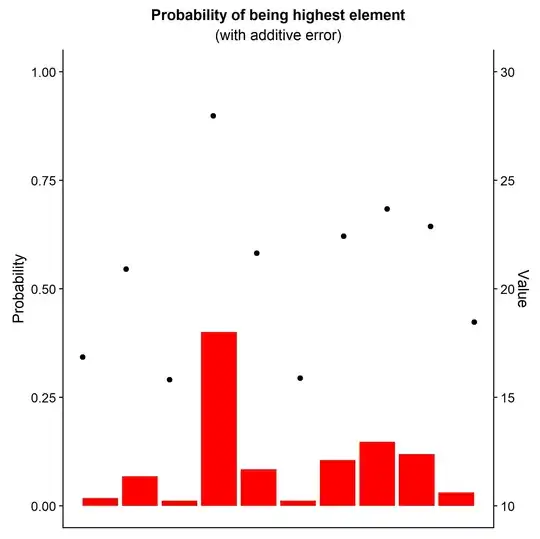
Theoretical formula

According to this calculating probabilities for two variables is simple:

$$P(A<B) = \Phi\left(\dfrac{\mu_B-\mu_A}{\sqrt{\sigma_A^2+\sigma_B^2}}\right)$$

If we look at the other link you will see a much more complicated formula for multiple variables (and it means that the maximum of variables are interdependent). $$P(X_1 > \max X_i) = \int_{-\infty}^{\infty}\prod_{i=2}^n \Phi\left(\frac{\alpha-\mu_i}{\sigma_i}\right) \frac{1}{\sigma}\phi\left(\frac{\alpha-\mu_1}{\sigma_1}\right)\,\mathrm d\alpha$$ Taking into account that $\Phi$ is itself an integral without a theoretical solutions we have a very complicated formula with n integrals in it.

Computational benchmarks

As proposed in the second link the probabilities could be calculated using Monte-Carlo simulations.

Here are the benchmarks for integration of the theoretical formula, Monte-Carlo simulations and Ben's numerical calculation. All in Python:

Number of variables = 100.  
Monte-Carlo simulations: 531 ms (100000 simulations) (gives correct answer)
Numerical calculation from Ben's answer: 22.1s (gives correct answer)  
Integration according to the theoretical formula: 23.3s (gives wrong answer)

All algorithms are adjusted to have precision of around 1e-3 for the last value (99)

With the first approach I got the sum of probabilities equal to 0.92. Either it is a problem with integration in Python or the theoretical formula is wrong. And I was not able to vectorize the code so it should be significantly slower than C. With simulations I was able to write vector functions in numpy so the time should be closer to C.

The accuracy of the simulation is calculated with standard deviations (for values 99,98 and 97 respectively):

mean probability = 7.2469e-01, std=1.13458614e-03
mean probability = 2.2255e-01, std=7.49851686e-04
mean probability = 4.6310e-02, std=1.07472256e-03
...

It may be possible to calculate the theoretical formula faster than the simulation by some good approximation of the integration. For example remove all variables that are 3 standard deviations from the maximum value, use piece-wise linear function for $\Phi$, and use few evaluations for numerical computation of the integral.

The code:

import numpy as np
from scipy.stats import norm
from scipy.integrate import quad

n=100
m = np.arange(100.)
sd = np.ones(100)

def func(x,m,sd,i):
    mul = 1/sd[i]*norm.pdf((x-m[i])/sd[i])
    for j in range(n):
        if i!=j:
            mul = mul*norm.cdf((x-m[j])/np.sqrt(sd[i]**2+sd[j]**2))
    return mul

Measuring execution time of the theoretical integration formula in jupyter:

%%time
prob = np.array([quad(func,-np.inf,m[i],args=(m,sd,i),epsabs=1e-3)[0]+quad(func,m[i],np.inf,args=(m,sd,i),epsabs=1e-3)[0] for i in range(n)])
# 23.3 s 

Measuring execution time of the Monte-Carlo simulations in jupyter:

%%time
nn=100000
a = np.random.normal(size=(n,nn))*sd[:,None]+m[:,None]
print((a==a.max(axis=0)).sum(axis=1)/nn)
# 531 ms

Calculating standard deviations:

nn=100000
a = np.random.normal(size=(n,nn,7))*sd[:,None,None]+m[:,None,None]
((a==a.max(axis=0)).sum(axis=1)/nn).std(axis=1)

Ben's numerical approach in R gives the same result as Monte-Carlo simulations. Here is the same code in Python that I used for benchmarking:

%%time
nn=25000
e_vec = np.random.normal(size=nn)
a = np.empty((n,nn))
i_range = np.arange(n)
for i in range(n):
    a[i]=np.prod(norm.cdf(m[i]-m[np.arange(len(m))!=i][:,None]+e_vec[None,:]), axis=0)
print(a.mean(axis=1))
#22.1s

Probabilities for values 99,98,97:

0.727, 0.225, 0.047

Code to calculate the standard deviation of Ben's numerical answer:

nn=25000
a4std = np.empty((7,n))
for ii in range(7):
    e_vec = np.random.normal(size=nn)
    a = np.empty((n,nn))
    i_range = np.arange(n)
    for i in range(n):
        a[i]=np.prod(norm.cdf(m[i]-m[np.arange(len(m))!=i][:,None]+e_vec[None,:]), axis=0)
    a4std[ii] = a.mean(axis=1)        
print(a4std.std(axis=0))

Standard deviation for values 99,98,97:

1.84e-3, 1.77e-3, 9.9e-4