How to fit laplace/exponential distribution to cosine similarities?

Question

I am a computational biologist with little experience fitting data.

I'm trying to fit a distribution of cosine similarities computed between sparse matrices. The goal is to be able use this distribution as a null distribution to compute p-values of computed cosine similarities on real data.

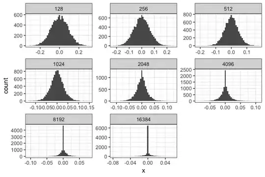
The null distribution of cosine similarities is typically assumed to follow a normal distribution because of the central limit theorem and indeed this is what we see when the vectors are dense.

However, in a biological setting we would more often deal with fairly sparse vectors (~95% 0’s) (in this case we're talking about gene membership to a geneset when the universe of genes increases). When we increase the sparsity of the vectors and plot the distribution of cosine similarities, we see that it rapidly becomes non-normal and inflated at 0. In our simulations, we keep the amount of non zero genes fixed and increase the total size of the vector (with the remaining genes being all 0)

Visually, it looks like the distribution moves from being gaussian to Laplace as sparsity increases. We've tried to fit this dataset using a double exponential (dlaplace from the package jmuOutlier) and the ideas from this post

x <- seq( min(mydata), max(mydata), length.out=20 )
mean_estimated <- median(mydata)
sd_estimated <- mean(abs(mydata-mean_estimated))
laplace_curve <- dlaplace(x, mean=mean_estimated, sd=sd_estimated )

res <- hist(mydata, breaks = 100)
plot(res$mids, res$counts)

hist(mydata, breaks = 100, freq = F) 
curve(dlaplace(x, mean=mean_estimated, sd=sd_estimated ), col = "red", add = TRUE)

and here's some sample data

my data <- c(0,0,0,-121.812475497063,-17.1317497626788,0,0,0,8.35572739928506,0,-26.9359145415957,20.4527916510325,0,-4.74715944618195,117.542381259887,232.123630295157,123.223331644106,0,363.307449720702,0,17.2876056009945,48.4743173227965,0,-59.3313238079675,72.1418015633871,26.6828781262261,0,-9.59200428642452,0,0,0,0,0,0,14.7726016702487,0,-325.332919994427,104.648601779681,-41.5876513726268,0,23.8977917597686,0,-4.61753733424316,0,-126.668971720393,1.45200133967801,0,-401.095618197396,16.7718497697131,0,0,361.956158574512,-0.041911914563271,0,0,-154.903446590557,-24.5034756181517,0,-46.4799574666324,0,-78.0146685968426,0,0,0,-12.7363529440765,0.801785045212923,79.7353310556848,263.50396219768,68.7207464247363,-16.6983607980076,0,0,0,0,9.49049366986621,0,-25.2709579790211,18.9158672257186,-16.5083502102244,-123.816047852029,0,10.074510523382,-1.7805270018387,-1.12260723072776,-34.5358930060155,112.65174921281,0,0,0,0,0,0,110.661061532395,-4.76648158660036,0,0,0,64.7388429927619,0,83.4665923262401,-90.5948140823812,48.1520353229011,83.2419061957572,84.6904132512109,-32.5771834489668,0,-24.4646160022276,0,0,16.283865284046,845.919876029546,0,0,30.9790913857609,-64.1857905888979,-71.8981992333845,0,0,-82.3833048984224,0,6.91280012973377,0,14.3260581532408,0,-88.4583037875095,4.81561616305259,0,0,0,0,224.936048456396,2.76354047838483,0,-12.3129795553901,0,0,202.221902345161,3.87903891367971,-6.78101669022923,0,-110.337466635902,0,0,-200.683877785148,0,-52.9434473377721,0,0,0,0,-55.5823775087446,204.412102111891,-89.7181809211675,160.514222115252,-43.1977265125341,-119.720898068799,360.198526060316,0,0,-73.5877173033978,0,0,0,0,0,85.2054592768861,63.8154881905621,-2.45087824145073,0,0,0,0,-36.787934899427,0,0,0,-49.62704298923,-12.549272621154,109.89567398325,0,-19.5206671407738,0,-84.0358460651716,-8.96146044988531,0,0,-40.9156265799148,0,0,88.0444551252554,0,0,23.6917582249244,-11.7178035932228,0,-2.54341767902909,0,63.3618229985467,0,0)

However, there's clearly an inflation in zero that we are not able to fit. Is there a better function suited to fit this type of distribution? Thanks in advance.

Answer 1

I fit the example data to just over 85 of the continuous distributions in scipy using my online statistical distribution fitter at http://zunzun.com/StatisticalDistributions/1/ and the best two candidates appear to be:

double Weibull distribution:
http://docs.scipy.org/doc/scipy/reference/generated/scipy.stats.dweibull.html

Fit Statistics for 200 data points:
    Negative Two Log Likelihood = -1.0547446143691981E+04
    AIC = -1.0541446143691981E+04
    AICc (Burnham and Anderson) = -1.0541323694712390E+04


Parameters:
    c = 1.7386724007711302E-01
    location = -6.2987003530715147E-34
    scale = 1.6198330950867783E+00

Additional Information:
The probability density function for `dweibull` is:

        dweibull.pdf(x, c) = c / 2 * abs(x)**(c-1) * exp(-abs(x)**c)

and

double gamma distribution
http://docs.scipy.org/doc/scipy/reference/generated/scipy.stats.dgamma.html

Fit Statistics for 200 data points:
    Negative Two Log Likelihood = -7.7257658319076218E+03
    AIC = -7.7197658319076218E+03
    AICc (Burnham and Anderson) = -7.7196433829280295E+03


Parameters:
    a = 2.8099490449925113E-01
    location = 3.3797498248908335E-30
    scale = 1.9451598451628075E+02

Additional Information:
The probability density function for `dgamma` is:

        dgamma.pdf(x, a) = 1 / (2*gamma(a)) * abs(x)**(a-1) * exp(-abs(x))

Answer 2

If your data has a lot of zeros in it, why not model its distribution as a mixture of a normal (or Laplace if you want) distribution and a spike at zero? I tried fitting your example data by maximum likelihood estimation, implemented directly in julia (but I'm sure this can be done in R too):

import PyPlot; plt=PyPlot # for plotting
using Optim # for optimization
using Distributions # probability distributions
my_data = [0,0,0,-121.812475497063,-17.1317497626788,0,0,0,8.35572739928506,0,-26.9359145415957,20.4527916510325,0,-4.74715944618195,117.542381259887,232.123630295157,123.223331644106,0,363.307449720702,0,17.2876056009945,48.4743173227965,0,-59.3313238079675,72.1418015633871,26.6828781262261,0,-9.59200428642452,0,0,0,0,0,0,14.7726016702487,0,-325.332919994427,104.648601779681,-41.5876513726268,0,23.8977917597686,0,-4.61753733424316,0,-126.668971720393,1.45200133967801,0,-401.095618197396,16.7718497697131,0,0,361.956158574512,-0.041911914563271,0,0,-154.903446590557,-24.5034756181517,0,-46.4799574666324,0,-78.0146685968426,0,0,0,-12.7363529440765,0.801785045212923,79.7353310556848,263.50396219768,68.7207464247363,-16.6983607980076,0,0,0,0,9.49049366986621,0,-25.2709579790211,18.9158672257186,-16.5083502102244,-123.816047852029,0,10.074510523382,-1.7805270018387,-1.12260723072776,-34.5358930060155,112.65174921281,0,0,0,0,0,0,110.661061532395,-4.76648158660036,0,0,0,64.7388429927619,0,83.4665923262401,-90.5948140823812,48.1520353229011,83.2419061957572,84.6904132512109,-32.5771834489668,0,-24.4646160022276,0,0,16.283865284046,845.919876029546,0,0,30.9790913857609,-64.1857905888979,-71.8981992333845,0,0,-82.3833048984224,0,6.91280012973377,0,14.3260581532408,0,-88.4583037875095,4.81561616305259,0,0,0,0,224.936048456396,2.76354047838483,0,-12.3129795553901,0,0,202.221902345161,3.87903891367971,-6.78101669022923,0,-110.337466635902,0,0,-200.683877785148,0,-52.9434473377721,0,0,0,0,-55.5823775087446,204.412102111891,-89.7181809211675,160.514222115252,-43.1977265125341,-119.720898068799,360.198526060316,0,0,-73.5877173033978,0,0,0,0,0,85.2054592768861,63.8154881905621,-2.45087824145073,0,0,0,0,-36.787934899427,0,0,0,-49.62704298923,-12.549272621154,109.89567398325,0,-19.5206671407738,0,-84.0358460651716,-8.96146044988531,0,0,-40.9156265799148,0,0,88.0444551252554,0,0,23.6917582249244,-11.7178035932228,0,-2.54341767902909,0,63.3618229985467,0,0]
n = length(my_data)

""" Create a spike-and-slab mixture distribution
    consisting of a Normal(μ, σ) slab
    and a narrow Normal(0, 0.001) spike.
"""
function spike_slab(μ, σ, pspike)
    mix = MixtureModel([Normal(μ, σ), Normal(0.0, 0.001)], # components
                       [1.0-pspike, pspike])               # weights
    return mix
end

logistic(x::Real) = inv(exp(-x) + one(x)) # inverse logit
function make_optim_target(data)
    function optim_target(θ)
        μ, logσ, logitp = θ
        if logσ < -5
            # don't bother
            return Inf
        end
        # obtain the distribution:
        mix = spike_slab(μ, exp(logσ), logistic(logitp))
        # compute the log-likelihood under this distribution
        ll = Distributions.loglikelihood(mix, data)
        return -ll # minus because Optim minimizes functions
    end
end

f_ll = make_optim_target(my_data) # generate the optimization function
init_x = [0.0, 0.0, 0.0]          # initial parameters
opt_out = Optim.optimize(f_ll, init_x, method=NelderMead()) # optimize!

# obtain the fitted distribution
μ, logσ, logitp = Optim.minimizer(opt_out)
mix = spike_slab(μ, exp(logσ), logistic(logitp))

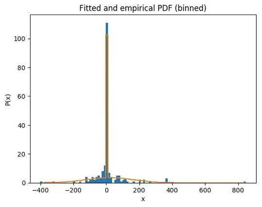
Now plotting the PDF:

counts, bins = plt.plt[:hist](my_data, bins=100)
mix_pmf = diff(cdf.(mix, bins))
plt.plt[:step](bins[2:end], mix_pmf .* n)
plt.title("Fitted and empirical PDF (binned)")
plt.xlabel("x")
plt.ylabel("P(x)")

and the CDF:

counts, bins = plt.plt[:hist](my_data, bins=100)
mix_pmf = diff(cdf.(mix, bins))
plt.plt[:step](bins[2:end], mix_pmf .* n)
plt.title("Fitted and empirical PDF (binned)")
plt.xlabel("x")
plt.ylabel("P(x)")

The sample data you shared has an outlier above 800, which is causing the fitted normal component to have a high standard deviation. It might make sense to either replace the normal component of the mixture with something that has fatter tails, or add a third very wide component. This can be done fairly easily starting from the code above.