I would say that the methods using 'maximum likelihood' and 'iterated reweighted least squares' are independent concepts. It is only in a specific case, the generalized linear model (GLM), that the two coincide.
The article speaks of two different type of derivations.
- One is the derivation done in the 70s by Nelder and Wedderburn, and in different forms by others, that linked GLM models with iterated reweighted least squares (IRLS).
- Another (the section 4 Unbinned maximum-likelihood from IRLS) is a derivation which is a bit different from the typical Iterated reweighted least squares. It is a derivation that shows that minimizing $\chi$ in Pearson's chi-squared method (by means of IRLS) coincides with maximizing the likelihood in the limit of the binsizes going to zero.
The "derivation" that is spoken about in the references (Wedderburn's work on GLM) is not a derivation of the maximum likelihood out of iterated reweighted least squares or vice versa.
That derivation is about proof of the equivalence between the two in a particular situation (in the case of generalized linear models).
I think that the below Venn diagram shows intuitively where these two methods coincide, and in which cases they differ. The methods are not the same (only for a specific subset are they the same, namely for GLMs). Therefore the methods are independent concepts that stand on their own and the one is not derived out of the other.
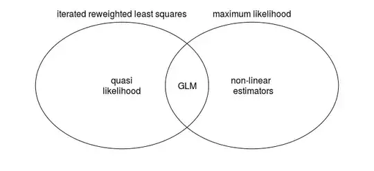
Iterated Reweighted Least Squares
The generalized least squares method, and related derived iterated reweighted least-squares (IRLS), stands on its own.
The motivation for this IRLS method is pragmatic: It is the best linear unbiased estimator. It is related to the Gauss–Markov theorem (and related to Aitken's extension). The variance of a linear estimator is independent from the specific error distribution, except the covariance matrix of the errors (and under the right circumstances some linear estimator, the leats squares solution, can be shown to have the lowest variance of all linear estimators).
(and so, because of that independence from the specific error distribution except for the variance, whenever ML coincides with a linear estimator, which is for GLMs, then the specific error distribution does not matter, and it is all about the variance of the error distribution only, and the two happen to give the same result)
Maximum Likelihood
Maximum likelihood also stands on its own.
The motivation for maximum likelihood is not something that was derived. It started out of ideas about inverse probability and fiducial probability (but without the Bayesian prior). As long as functions are 'well-behaved' then those principles/ideas/intuitions make sense and you get that MLE (or related estimates like bias-corrected estimates) are consistent and efficient.
The MLE, and likelihood, relate to some results that are independent from least-squares like Wilks theorem and the Cramer-Rao bound.
The maximum likelihood method is an independent principle and applied early in the history of statistical/probability thinking, before/independent from generalized least-squares methods.
- Difference with Least Squares
The maximum likelihood estimate extends to a larger region than what can be done with IRLS. Note that the Gauss Markov theorem and the generalized least squares relate specifically to linear estimators.
Example (Laplace distribution): Say, you estimate the location parameter of a Laplace distributed variable (which is not a GLM). In that case the sample median (maximum likelihood estimate) will be the minimum variance unbiased estimator (MVUE), which will be better than the sample mean (least-squares estimate), which is indeed the BLUE but not the MVUE.
So such a simple example already shows that there is more than just least squares estimation.
The Poisson distribution happens to be a special case where the BLUE is also MVUE. The $\lambda$ that minimizes the likelihood function happens to be the mean $\lambda = \frac{1}{n} \sum_{i=1}^n y_i$. The same thing is true for the normal distribution which happens to coincide with least-squares estimation (but least-squares is not a general principle that relates to any distribution).
The maximum likelihood estimate, or other estimates based in likelihood, is a more general principle that applies more widely than just those generalized linear models.
The equivalence between iterated reweighted least squares and maximum likelihood
In the article, it is mentioned that
the maximum-likelihood (ML) method can be derived a limiting case of an iterated weighted least-squares fit.
But I believe that this is in the wrong direction, or maybe none of the principles can be derived out of the other.
In your article, you refer to sources like
-
The iterated (re)weighted least-squares methods (IWLS or IRLS) are well
known in statistical regression [8]
J. A. Nelder, R. W. M. Wedderburn, Generalized Linear Models, J. R.
Statist. Soc. A135, 370–384 (1972).
Where the maximum likelihood is the starting point and IRLS is derived as a method to compute the maximum likelihood in the case of GLM problems.
-
Charles, Frome, and Yu [9] derived that the IWLS fit gives the exact same result as the ML fit for a family of distributions.
A. Charles, E.L. Frome, P. L. Yu, The Equivalence of Generalized Least
Squares and Maximum Likelihood Estimates in the Exponential Family, J.
Am. Stat. Assoc. 71, 169–171 (1976).
Where IRLS is the starting point and it is shown to be equivalent to ML only in the case of specific exponential models, namely GLM problems.
In Wedderburn 1974, this is extended further. You can take any IRLS as a starting point and turn it into a quasi-likelihood model. (and in the case of a single parameter distribution is the quasi likelihood function, derived from IRLS, the same as a true likelihood function).
The same article by Wedderburn shows how iterated reweighted least-squares is equivalent to the Gauss-Newton method of optimizing the likelihood function (and mentioned in Kjetil's answer).
About the article.
I find it confusing. I am not sure what the point is that it wants to make. You write
The insights discussed here are known in the statistics community [1, 2], but less so in the high-energy physics community.
It is admirable to explain the points from those two references. But which insights are being shared is not so clear to me. There seems to be a thing about computation speed differences (or the number of iterations, which is different than speed) and robustness differences (whatever that might mean) between using the iterated reweighted least squares method and the MIGRAD and MINUIT algorithms, but this is not made very clear (and my intuition tells me that IRLS is just like Gauss-Newton, also a straightforward minimizer of the likelihood, where it is not clear why this should be better than MIGRAD or MINUIT). Figure 1 shows something but I do not understand how it makes it more clear or whether it is even sufficient (heuristic) proof/indication.
About the derivation.
We start by considering a histogram of $k$ samples $x_i$. Since the samples are independently drawn from a PDF, the histogram counts $n_l$ are uncorrelated and Poisson-distributed. Following the IWLS approach, we minimize the function
$$Q( \mathbf{p} ) = \sum_l \frac{( n_l − kP_l )^2}{k \hat{P̂}_l}$$
and iterate, where $P_l ( \mathbf{p} ) = \int_{x_l}^{x_l + \delta x} f(x;\mathbf{p}) dx$ is the expected fraction of the
samples in bin $l$...
I do not see this as a typical iterated reweighted least-squares method where you only assume the variance as a function of the mean.
Instead, in this derivation, you use very explicitly the distribution density $f(x;\mathbf{p})$ as a starting point and not only the variance of the distribution as a function of mean of the distribution.
What you are basically doing is showing that a discretized version of likelihood maximization by histograms and by means of Poisson distribution for the distribution in the bins is asymptotically equal to a continuous likelihood maximization. (You are basically finding the distribution that optimizes Pearson's Chi-squared statistic and then take the limit of bin sizes to zero).
While it is an interesting derivation for the equivalence of the two, this is not really the typical iterated reweighted least squares method where you only need the variance of the distribution as a function of the mean of the distribution. What you do here is not a fitting of the (conditional) expectation, but instead a fitting of the entire probability density (by means of a histogram).
Iteratively minimizing the IRLS expression
$$Q( \mathbf{p} ) = \sum_l \frac{( n_l − kP_l )^2}{k \hat{P̂}_l}$$
Is equivalent to minimizing the related loss function
$$L( \mathbf{p} ) = \sum_l P_l + \frac{ n_l}{k} \log P_l $$
or since $ \sum_l P_l$ is constant
$$L( \mathbf{p} ) = \sum_l \frac{ n_l}{k} \log P_l $$
So you presuppose some sort of likelihood or goodness of fit and just use IRLS (optimizing $L$ by iteratively optimizating $Q$) to compute an optimal most likely fit of the data with the distribution function. This is not really like maximum likelihood is derived from IRLS. It is more like maximum likelihood is derived from the decision to fit the distribution function $f(x;\mathbf{p})$.
