First, you must realize that precision, accuracy, efficiency, and consistency are technical terms. Ordinary English words have been chosen for each concept because someone thought they were memorable and appropriate, and then a formal
definition is given. Once the formal definition is given, that definition is what matters--not what any one person thinks the original English word ought to mean.
Your examples of accuracy and precision are pretty good. Let's take a slightly more formal look at those two terms as a start:
Accuracy and biasedness. Accuracy means small bias. As an estimator of a normal population mean $\mu,$ the sample mean $\hat \mu = \bar X$ is unbiased. That is, $E(\bar X) = \mu.$ The bias of an estimator $\hat \theta$ of a parameter $\theta$ is defined as $B(\hat \theta) = E(\hat \theta - \theta).$ Because $E(\bar X - \mu) = 0,$ we say that $\bar X$ is an unbiased estimator of $\mu.$
Precision and variance: However, the sample mean $\bar X$ is not the only unbiased estimator of the normal mean $\mu.$ One can prove that the sample median $\widetilde X$ is also unbiased. When we know the data are sampled from a normal population, we usually use the sample mean $\bar X$ instead of the sample median $\widetilde X$ because the sample mean $\bar X$ is more precise. The precision $\tau_{\hat\theta}$ of an estimator $\hat \theta$ is defined as the reciprocal $\tau_{\hat\theta} = \frac{1}{{\sigma_{\hat\theta}}^2}$ of its variance.
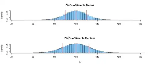
Based on a million random samples of size $n = 25$ from $\mathsf{Norm}(\mu=100,\, \sigma=15),$ here are approximate distributions of sample means a and sample medians h, as computed in R. Notice that $E(\bar X) = E(\widetilde X) = 100,$
but $Var(\bar X) = \sigma^2/n = 25 < Var(\widetilde X).$
set.seed(721);  m = 10^6; n = 9;  mu = 100; sg = 15
a = replicate(m, mean(rnorm(n, mu, sg)))
mean(a); sd(a)
[1] 100.0022   # aprx E(A) = 100
[1] 4.999926   # aprx SD(A) = 5
set.seed(721)  # same one million samples again
h = replicate(m, median(rnorm(n, mu, sg)))
mean(h); sd(h)
[1] 100.0068   # aprx E(H) = 100
[1] 6.108649   # aprx SD(H) > SD(A)
The figure below shows histograms of the million sample means (top) and the
million sample medians. Vertical lines show the location of the mean and one
standard deviation on either side of the mean. Clearly, the sample mean has higher precision (smaller variances) as an estimator of $\mu$ than does the sample median.
Consistency and sample size: An estimator $\hat \theta_n$ (based on $n$ observations) of parameter $\theta$ is called consistent if $\hat \theta_n \stackrel{prob}{\rightarrow} \theta,$ as $n \rightarrow \infty.$ Technically,
'convergence in probability` means that
$\lim_{n \rightarrow \infty} P(|\hat \theta_n - \theta| < \epsilon) = 1,$ for any $\epsilon > 0.$ [We can't speak in terms of 'ordinary' convergence of $\hat \theta_n$ because each $\hat\theta_n$ is an unknown random quantity. However, for a given $\epsilon > 0,$ we can
speak of convergence of $Q_n = P(|\hat \theta_n - \theta| < \epsilon)$ because
each $Q_n$ is a computable probability based on the population distribution.]
A rough intuitive statement is that the error of the estimate shrinks to $0$ as sample size increases. In the simulation above, $n = 25$
observations gave values of $\bar X$ within $\pm 10$ units most of the time.
With a larger sample size $n$ the errors would tend to be smaller. The
sample median is also a consistent estimator of $\mu,$ but for any given $n$ the sample mean is preferable because of its greater precision.
Efficiency and criteria: Before evaluating the 'goodness' of an estimator, we need to know what we mean by 'good'. Above we have mentioned 'accuracy' and 'precision' as desirable properties of an estimator. But there are slightly biased estimators that are quite good for some purposes, and unbiased estimators that are essentially useless.
For example, for normal data the sample standard deviation $S$ has $E(S) < \sigma.$ (The bias is moderate for small $n$ and negligible for large $n.$ See this Q & A.)
set.seed(721);  m = 10^6; n = 5;  mu = 100; sg = 15
s = replicate(m, sd(rnorm(n, mu, sg)));  mean(s)
[1] 14.10341
One commonly used criterion is to minimize
$$MSE = E[(\hat\theta - \theta)^2] = Var(\hat\theta) + [B(\hat\theta)]^2.$$
If an estimator satisfies such a criterion, then it is called efficient (relative to the criterion). One can show that the sample mean is MSE efficient when sampling from a normal distribution. Obviously, the sample median is not efficient because both the sample mean and the sample median are unbiased, and the median has a larger variance, thus a larger MSE. (For a more detailed and technical discussion see Wikipedia on 'Efficient statistic' and other links form there.)
