4

I'm trying to change negative values to positive from my linear model.

Here is my attempt:

dist <-
c(2, 2.1, 2.21, 2.31, 2.41, 2.52, 2.62, 2.72, 2.83, 2.93, 3.03,
3.14, 3.24, 3.34, 3.45, 3.55, 3.66, 3.76, 3.86, 3.97, 4.07, 4.17,
4.28, 4.38, 4.48, 4.59, 4.69, 4.79, 4.9, 5)

accuracy <-
c(0.13, 1.21, 2, 0.78, 0.4, 1.47, 0.28, 2.18, 0.74, 0.51, 1.12,
0.48, 1.71, 3.35, 1.36, 0.95, 0.78, 3.51, 0.24, 5, 3.25, 4.29,
7.33, 4.12, 20.25, 7.05, 36.25, 2.78, 14.93, 13.45)

> summary(lm(glm(log(accuracy)~log(dist))))

Call:
lm(formula = glm(log(accuracy) ~ log(dist)))

Residuals:
 Min       1Q   Median       3Q      Max 
-2.57614 -0.72039  0.02401  0.56570  1.73818 

Coefficients:
        Estimate Std. Error t value Pr(>|t|)    
(Intercept)  -3.7278     0.8123  -4.589 8.52e-05 ***
log(dist)     3.6107     0.6513   5.544 6.29e-06 ***
---
Signif. codes:  0 ‘***’ 0.001 ‘**’ 0.01 ‘*’ 0.05 ‘.’ 0.1 ‘ ’ 1

Residual standard error: 0.9594 on 28 degrees of freedom
Multiple R-squared:  0.5233,    Adjusted R-squared:  0.5062 
F-statistic: 30.73 on 1 and 28 DF,  p-value: 6.291e-06

I've used the logarithm to try make the intercept a positive number, but I still get a negative.

How do I make the intercept a positive number?
Glorfindel
  • 700
  • 1
  • 9
  • 18

2 Answers2

8

The estimated intercept coefficient in your log-linear model is negative because your line-of-best fit has an accuracy intercept that is less than one (which corresponds to a negative logarithm). There is nothing wrong with this; that is what the line-of-best-fit for this model looks like. (If you really want to change the intercept estimate to be positive, you could change to a logarithmic scale with a small base, which would scale your intercept up by a corresponding constant. This would add nothing of substance to the analysis, and I would not recommend it.)

Remember that a negative intercept on a log-scale still gives you a non-negative value for the underlying response variable. From your model you have the regression line:

$$\ln (\hat{\text{acc}}) = -3.7278 + 3.6107 \cdot \ln(\text{dist}).$$

Reversing the logarithm yields the corresponding regression equation:

$$\hat{\text{acc}} = \exp (-3.7278) \cdot \text{dist}^{3.6107} = 0.02404615 \cdot \text{dist}^{3.6107}.$$

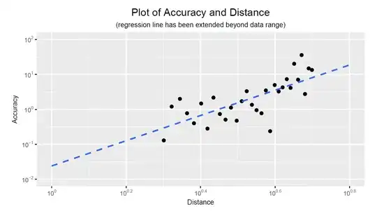
In the case corresponding to the intercept term you have where $\text{dist} = 1$ (so that $\ln (\text{dist}) = 0$) which gives $\ln (\hat{\text{acc}}) = -3.7278$, so that the predicted response is $\hat{\text{acc}} = 0.02404615$. This intercept value for your line-of-best-fit can be seen easily in a scatterplot of your data, displayed on a log-10 scale (R code for the plot shown below).

enter image description here

DATA <- data.frame(Accuracy = accuracy, Distance = distance);

library(ggplot2);

ggplot(data = DATA, aes(x = Distance, y = Accuracy)) +
       geom_point(size = 2) + 
       geom_smooth(method = 'lm', formula = y ~ x, se = FALSE, 
                   fullrange = TRUE, linetype = "dashed") +
       scale_y_log10(breaks = trans_breaks("log10", function(x) 10^x),
                     labels = trans_format("log10", math_format(10^.x)),
                     limits = c(10^(-2), 10^2)) +
       scale_x_log10(breaks = trans_breaks("log10", function(x) 10^x),
                     labels = trans_format("log10", math_format(10^.x)),
                     limits = c(10^0, 10^(0.8))) +
       ggtitle("Plot of Accuracy and Distance") +
       labs(subtitle = "(regression line has been extended beyond data range)") +
       xlab("Distance") + ylab("Accuracy");
Ben
  • 91,027
  • 3
  • 150
  • 376
4

This isn't a complete answer, but the graph won't fit in a comment. As implied by @Ben in his helpful answer, you are in effect trying to fit a power function or power law in accuracy $y$ as a function of dist $x$, that is $y= ax^b$, by fitting a straight line to log $y$ in terms of log $x$.

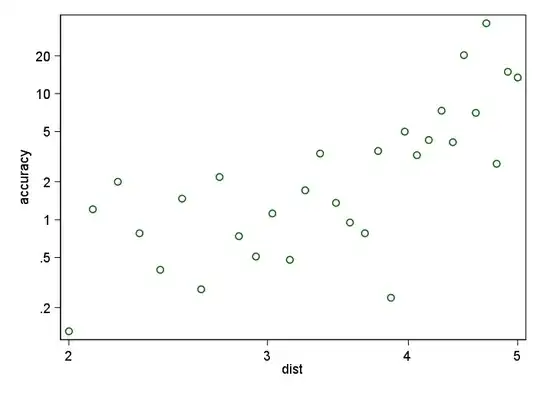
enter image description here

A graph of your data on logarithmic scales (above) implies that an estimate of $a$, which is the prediction for dist at $x = 1$, will be much smaller than $1$, so its logarithm will be smaller than $0$ with any commonly used base(*). But negative logarithms aren't unacceptable or problematic in themselves; they mean, with such bases, positive numbers $< 1$.

Whether a power law makes sense or can be well fitted with these data are bigger questions. The small moral is that plotting your data can help you see what is going on.

(*) EDIT: That corrects a mathematical slip pointed out by @whuber. It's a common but not essential convention that the base of logarithms is greater than 1, as is true for 10, $e = \exp(1)$ and 2.

Nick Cox
  • 48,377
  • 8
  • 110
  • 156
  • 1
    +1. (Tiny nitpick: by using a logarithmic base between $0$ and $1,$ the estimated intercept will indeed be positive! Therein lies a solution to the question as asked.) – whuber May 16 '18 at 11:16
  • 1
    @whuber Good point Edited. – Nick Cox May 16 '18 at 12:02