With binary predictors and a binary outcome, there are only 4 cells (conditions, or possibilities) to display: predictor = either 0 or 1 and outcome = either 0 or 1. Thus one can use a very simple format like a table or bar chart to show the connections between the two variables.
With a continuous predictor, the relationship may be more complex. One effective way to display this is through a sunflower plot.
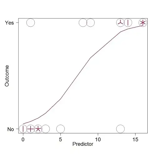
Each circle represents one case, and each sunflower "petal" represents an additional case that has the same Predictor and Outcome values as the rest of the cases in that circle.
With such a chart one can see exactly how many cases have each pair of values; to what extent the relationship departs from a linear one; and where the slope discriminating between "No" and "Yes" outcomes is steepest.
    # See http://stat.ethz.ch/R-manual/R-patched/library/graphics/html/sunflowerplot.html

require(stats); require(grDevices); library(lattice)

x=c(0,0,1,1,1,1,1,2,2,2,2,2,3,5,8,9,13,13,13,13,14,14,16,16,16,16,16,16)
y=c(0,0,0,1,0,0,0,0,0,0,0,0,0,0,1,1,1,1,1,0,1,1,1,1,1,1,1,1)
d=data.frame(x,y)

model = glm(y~x, family=binomial) ; fitted=predict(model, type="response")

sunflowerplot(x,y, rotate = F,  cex = 5, cex.fact = 1,  pch = 1,  yaxt = 'n', xlab='', ylab='',
   cex.axis=1.4,  col = "maroon",  seg.col = "maroon",  seg.lwd = 3)
title(xlab='Predictor', ylab='Outcome', line=2, cex.lab=1.4)
# line=2 determines axis title's distance from axis
axis(2, at= c(0,1), las = 1, labels=c('No', 'Yes'), cex.axis=1.4, cex.lab=1.4)
lines(x, fitted(model),col= "maroon", lwd = 1.7)

# Alt ways to get fitline
lines (lowess(y~x), lwd=2, col= "red")
lines (scatter.smooth(y~x), lwd=2)

# cex = size of plotted points
# size = petal size; 1/8 may work, or skip
# cex.fact = shrinkage ratio (points shrink compared to petals)
# seg.col = petal color
# seg.lwd = petal line width
# par(las=1) or simply "las=1" within a command will make axis labels horizontal
As for 'beta' and 'exponential(beta)', any general source on logistic regression will explain the difference, but in short: with the latter one raises beta to a power (the coefficient), base e. This yields the odds ratio associated with a case being 1 higher than another on the predictor. For example, when Music is '1' the odds of the outcome being '1' are 1.6 times the odds when Music is '0'.


