For 86 companies and for 103 days, I have collected (i) tweets (variable hbVol) about each company and (ii) pageviews for the corporate wikipedia page (wikiVol). The dependent variable is each company's stock trading volume (stockVol0). My data is structured as follows:
company  date  hbVol    wikiVol   stockVol0  comp1  comp2 ... comp89  marketRet
-------------------------------------------------------------------------------
1        1     200        150     2423325      1      0   ...   0     -2.50
1        2     194        152     2455343      1      0   ...   0     -1.45
.        .      .          .         .         .      .   ...   .
1       103    205        103     2563463      1      0   ...   0      1.90
2        1     752        932     7434124      0      1   ...   0     -2.50
2        2     932        823     7464354      0      1   ...   0     -1.45
.        .      .          .         .         .      .   ...   .
.        .      .          .         .         .      .   ...   .
86      103     3          55      32324       0      0   ...   1      1.90
As I understood, this is called pooled cross-sectional time series data. I have taken the Log-value of all variables to smoothen the big differences between companies. A regression model with both independent variables on the dependent stockVolo returns:
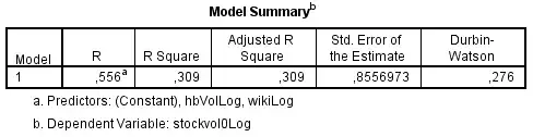
A Durbin-Watson of 0,276 suggest significant autocorrelation of the residuals. The residuals are, however, bellshaped, as can be seen from the P-P plot below. The partial autocorrelation function shows a significant spike at a lag of 1 to 5 (above upper limit), confirming the conclusions drawn from the Durbin-Watson statistic:
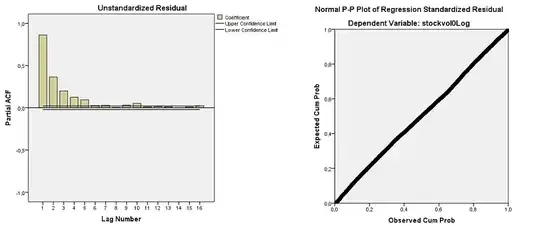
The presence of first-order autocorrelated residuals violates the assumption of uncorrelated residuals that underlies the OLS regression method. Different methods have been developed, however, to handle such series. One method I read about is to include a lagged dependent variable as an independent variable. So I created a lagged stockVol1 and added it to the model:
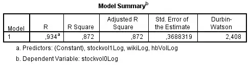
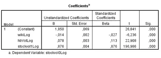
Now, Durbin-Watson is at an accceptable 2,408. But obviously, R-squared is extremely high because of the lagged variable, see also the coefficients below:
Another method I read about when being confronted with autocorrelation, is autoregression with Prais-Winsten (or Cochrane-Orcutt) method. Once performing this the model reads:
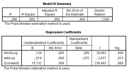
This is what I don't understand. Two different methods, and I get very different results. Other suggestions for analyzing this data include (i) not including a lagged variable but reformat the dependent variable by differencing (ii) perform AR(1) or ARIMA(1,0,0) models. I haven't calculated those because I am now lost on how to proceed because of the different results of the two tests I did perform.
What model should I use to perform a proper regression on my data? I'm very keen on understanding this, but have never had to analyze a timeseries dataset like this before.
 and
and 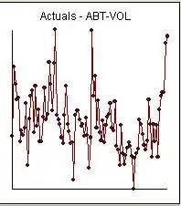 and
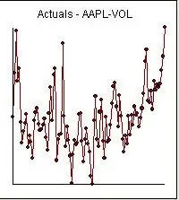
and 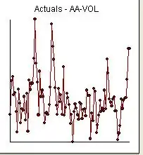 . Since anomalies are present the appropriate regression needs to take into account these effects. Following are the three models ( including any necessary lag structures in the two inputs ) and the appropriate ARIMA structure obtained from an automatic transfer function run using AUTOBOX ( a piece of software I have been developing for the last 42 years )
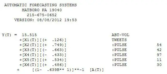 and
and 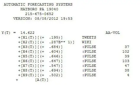 and
and 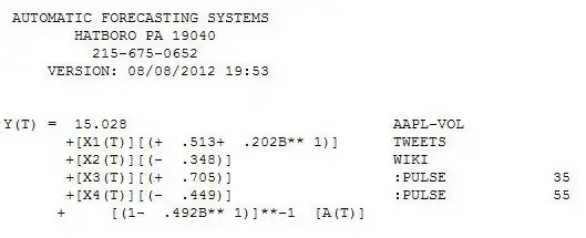 . We now take the three cleansed series returned from the modelling process and estimate a minimally sufficient common model which in this case would be a comtemporary and 1 lag PDL on tweets and a contemporary PDL on wiki with an ARIMA of (1,0,0)(0,0,0). Estimating this model locally and globally provides insight as to the commonality of coefficients .
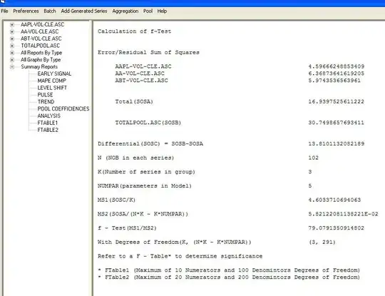 with coefficients
 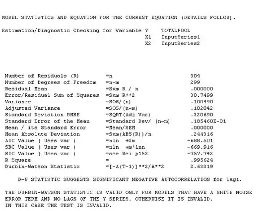 . The test for commonality is easily rejected with an F value of 79 with 3,291 df. Note that the DW statistic is 2.63 from the composite analysis. The summary of coefffici
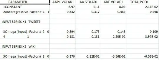 ents is presented here. The OP poster reflected that the only software he has access to is insufficient to be able to answer this thorny research question.