I am attempting to test some sets of data for normality. I have 64 groups to test. Each group has n=8 samples. [[I am aware of the problems with low n in regard to normality testing]]
My end goal is to be able to test these groups against one another with a t.test() (or similar) to determine if they are significantly different from one another.
As an example from one of the groups:
x=(-82.13 -77.00 -76.80 -75.35 -74.88 -74.65 -70.93 -70.61)
To start with I have used a shapiro-wilk test (shapiro.test()) and received p value 0.462 >0.05, and W = 0.923 (I cannot reject the null hypothesis that this data is from a normal distb). I have also created histograms of each groups data.
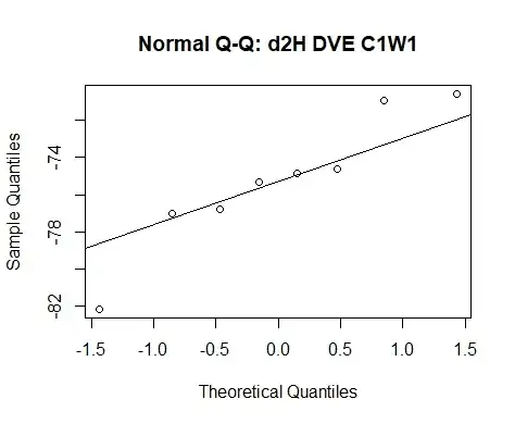
Then I use qqplot(x) and qqline(x) and get this result:

This method/approach is what I commonly find when reading how to carry out QQ-plots online.
However, I was taught a different method in my stats class. The following is the code for the alternative method:
v.h.c1w1Data <- sort(v.w1c1h) #Sort samples
v.h.c1w1Rank <- seq(1:length(v.w1c1h)) #Provide rank for each data point
v.h.c1w1F <- v.h.c1w1Rank/(length(v.w1c1h)+1) #Calculate the empirical prblty.
v.h.c1w1Mean <- mean(v.w1c1h)
v.h.c1w1Std <- sd(v.w1c1h)
v.h.c1w1Var <- var(v.w1c1h)
v.h.c1w1Model <- qnorm(v.h.c1w1F,v.h.c1w1Mean,v.h.c1w1Std) #calculate mdl prblty
qqplot(v.h.c1w1Data,v.h.c1w1Model, main= "Normal Q-Q: d2H DVE C1W1",xlab="d2H data (permil)", ylab="d2H modelled")
abline(0,1)
The result is the following plot.

My Question is: Since the 2 plots are clearly different and I think would be interpreted differently, which method is appropriate and why?