There would be no problem if $X$ were orthonormal. However, the possibility of strong correlation among the explanatory variables should give us pause.
When you consider the geometric interpretation of least-squares regression, counterexamples are easy to come by. Take $X_1$ to have, say, almost normally distributed coefficients and $X_2$ to be almost parallel to it. Let $X_3$ be orthogonal to the plane generated by $X_1$ and $X_2$. We can envision a $Y$ that is principally in the $X_3$ direction, yet is displaced a relatively tiny amount from the origin in the $X_1,X_2$ plane. Because $X_1$ and $X_2$ are nearly parallel, its components in that plane might both have large coefficients, causing us to drop $X_3$, which would be a huge mistake.
The geometry can be recreated with a simulation, such as is carried out by these R calculations:
set.seed(17)
x1 <- rnorm(100)               # Some nice values, close to standardized
x2 <- rnorm(100) * 0.01 + x1   # Almost parallel to x1
x3 <- rnorm(100)               # Likely almost orthogonal to x1 and x2
e <- rnorm(100) * 0.005        # Some tiny errors, just for fun (and realism)
y <- x1 - x2 + x3 * 0.1 + e
summary(lm(y ~ x1 + x2 + x3))  # The full model
summary(lm(y ~ x1 + x2))       # The reduced ("sparse") model
The variances of the $X_i$ are close enough to $1$ that we can inspect the coefficients of the fits as proxies for the standardized coefficients. In the full model the coefficients are 0.99, -0.99, and 0.1 (all highly significant), with the smallest (by far) associated with $X_3$, by design. The residual standard error is 0.00498. In the reduced ("sparse") model the residual standard error, at 0.09803, is $20$ times greater: a huge increase, reflecting the loss of almost all information about $Y$ from dropping the variable with the smallest standardized coefficient. The $R^2$ has dropped from $0.9975$ almost to zero. Neither coefficient is significant at better than the $0.38$ level.
The scatterplot matrix reveals all:
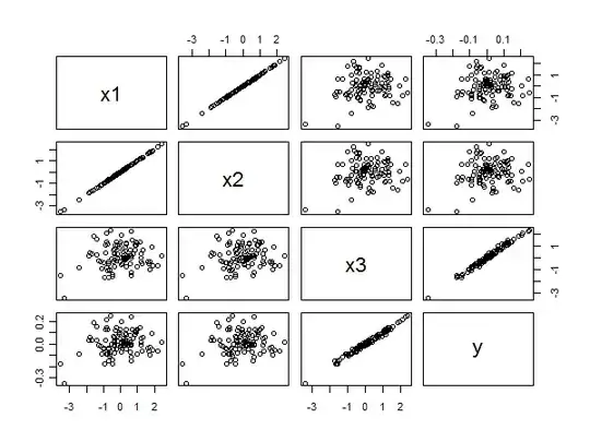
The strong correlation between $x_3$ and $y$ is clear from the linear alignments of points in the lower right. The poor correlation between $x_1$ and $y$ and $x_2$ and $y$ is equally clear from the circular scatter in the other panels. Nevertheless, the smallest standardized coefficient belongs to $x_3$ rather than to $x_1$ or $x_2$.