13

Suppose we have a set of points $\mathbf{y} = \{y_1, y_2, \ldots, y_N \}$. Each point $y_i$ is generated using distribution $$ p(y_i| x) = \frac12 \mathcal{N}(x, 1) + \frac12 \mathcal{N}(0, 10). $$ To obtain posterior for $x$ we write $$ p(x| \mathbf{y}) \propto p(\mathbf{y}| x) p(x) = p(x) \prod_{i = 1}^N p(y_i | x). $$ According to Minka's paper on Expectation Propagation we need $2^N$ calculations to obtain posterior $p(x| \mathbf{y})$ and, so, problem becomes intractable for large sample sizes $N$. However, I can't figure out why do we need such amount of calculations in this case, because for single $y_i$ likelihood has the form $$ p(y_i| x) = \frac{1}{2 \sqrt{2 \pi}} \left( \exp \left\{-\frac12 (y_i - x)^2\right\} + \frac{1}{\sqrt{10}} \exp \left\{-\frac1{20} y_i^2\right\} \right). $$

Using this formula we obtain posterior by simple multiplication of $p(y_i| x)$, so we need only $N$ operations, and, so we can solve this problem for large sample sizes exactly.

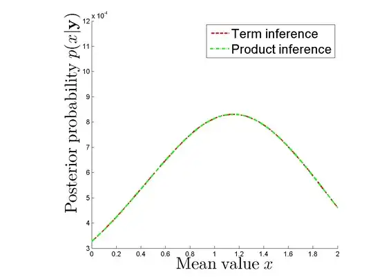
I make numerical experiment to compare do I really obtain the same posterior in case I calculate each term separately and in case I use product of densities for each $y_i$. Posteriors are same. See enter image description here Where am I wrong? Can anyone make it clear to me why do we need $2^N$ operations to calculate posterior for given $x$ and sample $\mathbf{y}$?

Alexey Zaytsev
  • 2,335
  • 15
  • 26
  • One operation per term and $N$ terms, so we need $O(N) $ operations. Also, I look through Minka's paper and Bishop's chapter on approximate inference again. Both suggest that we want estimate and obtain posterior for $x$. – Alexey Zaytsev Jul 14 '12 at 13:02
  • Am i understanding correctly that your $y_i$'s are univariate? If so, you can solve this in $O(n\log(n))$ which is considered tractable regardless of $n$ – user603 Jul 14 '12 at 13:28
  • 1
    @Alexey After re-reading this paragraph, I think the author does not mention $2^N$ operations. He just points out that **"the belief state for $x$ is a mixture of $2^N$ Gaussians"**. –  Jul 14 '12 at 13:46
  • 1
    @Procrastinator according to paper we want to use belief propagation, but can't use because we need to proceed mixture of $2^N$ gaussians. Then the question is why do we want to use BP? Another question arises in case we read chapter 10.7.1 in Bishop's PRML or watch [videolecture by Minka](http://videolectures.net/mlss09uk_minka_ai/). After that the answer isn't this clear. – Alexey Zaytsev Jul 14 '12 at 13:49
  • 1
    @Alexey I think the logic behind this is different. The author describes what happens if you use belief propagation, in order to emphasise some difficulties with it when $N$ is large, and then promoting his "expectation propagation". He mentions that belief propagation requires the use of a mixture of $2^N$ Gaussians for the belief state for $x$ which becomes complicated when $N$ is large. There is no mention to the number of operations required but to the complexity of the belief state for $x$. –  Jul 14 '12 at 13:55
  • @Procrastinator I think you are right after all, but I hope there exists a more explanatory example for EP, because this one looks a little far-fetched. – Alexey Zaytsev Jul 14 '12 at 13:58

2 Answers2

4

You are right that the paper is saying the wrong thing. You certainly can evaluate the posterior distribution of $x$ at a known location using $O(n)$ operations. The problem is when you want to compute moments of the posterior. To compute the posterior mean of $x$ exactly, you would need $2^N$ operations. This is the problem that the paper is trying to solve.

Tom Minka
  • 6,610
  • 1
  • 22
  • 33
2

You missed the point that the distribution is a mixture of Gaussians: each sample $y_i$ is either distributed as per $p(y_i | x)$ with probability $1-w$ and as $p_c(y)$ (clutter distribution for $y$, independent of $x$) with probability $w$.

Let $c_i$ be the indicator variable indicating that sample $i$ was draw from the clutter distribution; thus, if it's $0$ it indicates that the sample was drawn from $p(y|x)$. Obviously, if the sample was drawn from the clutter distribution it's value is irrelevant for the estimation of $x$.

It's the presence of the $2^N$ possible joint states for these indicator variables that causes the problem.

Dave
  • 3,109
  • 15
  • 23
  • However, we can drop additional $c_i$ variables, because we need to obtain a maximum posterior solution of the problem. Posterior for $x$ has a clear form, so we are not forced to take into account all $2^N$ present states. So, the question is "Why do we need this amount of computations in case we want to find a maximum posterior solution?" – Alexey Zaytsev Dec 08 '12 at 08:44
  • The maximization needs to be taken over the states for the $c$ variables. – Dave Dec 08 '12 at 22:59
  • We don't know $c_i$, so we integrate out (sum up over) $c_i$. This can be done in a direct way, doesn't it? – Alexey Zaytsev Dec 09 '12 at 14:20
  • Direct yes, but the number of states (terms) grows like $2^N$, which can be computationally problematic. – Dave Dec 10 '12 at 13:41
  • We can do this for each observation in an independent way, so we have $O(n)$, not $O(2^n)$ complexity. – Alexey Zaytsev Dec 11 '12 at 08:06
  • That amounts to a "mean field" approximation. – Dave May 23 '13 at 12:21