Correcting sample bias

Question

I am studying the correlation of two observed variables (call them $A$ and $B$). the underlying distribution for $A$ is symmetric around $0$ (for sure), however in my sample I have $411$ observations where it is negative and $470$ where it is positive due to sample bias.

Is it a correct way to remove the bias to simply filter out $470-411 = 59$ random positive observations from variable $A$ and the corresponding observations of variable $B$ before carrying on my analysis? This would rebalance the distribution of observations for $A$.

Ok, let's take an absurd example to make my point. Suppose you have a process following a perfect normal distribution centered at 0. A student draws 10000 samples one at the time and writes down the result. However, for reasons known only to her, she likes to write all the positive results on sheets of red paper and all the negatives on sheets of violet paper. If she can write 100 numbers on each sheet, at the end she will have roughly 50 red sheets and 50 violet sheets. She takes back all the sheet to her office desk to carry on the analysis but something terrible happens: a mutant paper-eating creature attacks her and eats only 23 of her violet sheets (the creature despises red paper). Now she has still around 50 red sheets, ie. around 5000 positive numbers, but only around 27 violet sheets, ie. 2700 negative numbers. She cannot repeat the experiment. What can she do? Can she choose randomly 23 red sheets and throw them away to rebalance the samples?

Answer 1

I will demonstrate that this effort at bias removal can, at least under certain (realistic) circumstances, introduce substantial bias. The demonstration is done with a simulation.

---

The answer depends on how the sample was obtained, the structure of the data, and what analyses will be performed. To make progress and to put this question into the usual framework, let's assume all $470+411$ observations are independently sampled from a common population (an iid sample).

First of all, the discrepancy between $411$ and $470$ could easily be due to chance. For variable $A$, being positive is an event with a $50%$ chance, whence (due to the independence of the observations) its count follows a binomial distribution with parameters $411+470$ and $0.5$. The chance of observing $470$ or more values of $A$ having a common sign is 5.06%: not terribly unlikely and not sufficient evidence to conclude the randomization failed. Ergo, there is no sampling bias.

However, isn't it intuitively obvious that the proposal to remove the excess data randomly in order to equalize the numbers of positive and negative $A$'s will not bias the sample? Although it makes sense, unfortunately it's not true.

As an example of what can go wrong, imagine yourself in the position of a consultant who recommends sampling procedures to scientists. The one being recommended here seems to be the following:

1. Randomly and independently draw $411+470$ individuals from the population.

2. If there is an excess of positive values of $A$ in the sample, randomly remove any individuals with positive values of $A$ in order to make the counts of positive and negative values equal. If there is an excess of negative values, follow a similar procedure to remove them.

3. Perform all subsequent analyses with the remaining data as if they formed an iid sample of the population.

Step 3 is a mistake. The resulting sample is not iid. Often it behaves very much like an iid sample, but not always. Suppose, for instance, that $B$ is a measurement of an (unobserved) attribute closely correlated with $A$: in fact, the unobserved attribute is believed to be a multiple of $A$ plus some unknown constant. However, the measurement is so crude that all it can indicate is whether that variable is positive or negative: this is what $B$ tells us. It is desired to test whether this underlying attribute has zero mean. The test will be based on the difference between the number of positive $B$'s and the number of negative $B$'s. (This is about the best possible test under the circumstances.)

Hypothesis tests rely on computing the expectation of a test statistic and the amount by which the statistic may vary: its sampling variance. If, for instance, $A$ has a normal distribution (of zero mean of course), then for an iid sample of size $411+470$, $B$ should range between $-100$ and $100$ and about $50%$ of the time it should lie between $-19$ and $19$. However, applying the "bias removal" procedure changes this. The reason is evident: in most random samples there will be an imbalance in the numbers of positive and negative values of $A$ by chance alone. If $B$ is strongly correlated with $A$, then it, too, will tend to have a similar imbalance. The "bias removal" process of balancing $A$ thereby approximately balances $B$. This causes $B$ to vary much less than one would expect.

Because this is a subtle phenomenon, detailed study is warranted. Interested readers might want to experiment with a simulation. Here is some R code. First, a function to "remove the bias":

filter <- function(x,y) {
  #
  # Randomly remove some (x,y) values in order to 
  # balance the numbers of positive and negative x's.
  #
  plus <- x > 0
  n <- length(x)
  n.plus <- length(x[plus])
  n.minus <- n - n.plus
  if (n.plus > n.minus) {
    omit <- sample(which(plus), n.plus-n.minus)
  }
  else {
    omit <- sample(which(x <= 0), n.minus-n.plus)
  }
  if (length(omit) > 0) {
    cbind(x,y)[-omit,]
  } else cbind(x,y)
}

Next, a function to convert values into a binary indicator of their sign so we can simulate $B$ exactly as described:

ind <- function(x) {
  y <- x*0
  y[x > 0] <- 1
  y
}

Now we can implement one iteration of the sampling process. The last argument, control, determines whether the "bias removal" is not or is applied.

trial <- function(n, rho, control=FALSE) {
  x <- rnorm(n)                            # `A` has a normal distribution
  y <- rnorm(n) * sqrt(1-rho^2) + rho * x  # Correlation coefficient is `rho`
  if (control) cbind(x,ind(y)) else filter(x,ind(y))
}

The statistical analysis tracks the net number of positive values of $B$:

stat <- function(y) {
  2 * length(which(y>0)) - length(y)
}

Finally, we can replicate the sampling many times to understand what will happen in the long run:

rho <- 0.9       # Correlation between `A` and the variable underlying `B`
n.trials <- 5000
sample.size <- 470+411
set.seed(17)
sim <- replicate(n.trials, apply(trial(sample.size, rho), 2, stat))
sim.control <- replicate(n.trials, apply(trial(sample.size, rho, control=TRUE), 2, stat))

A plot of the output clearly shows how the test statistic for $B$ varies much less than expected:

plot(sort(sim.control[2,]+rnorm(n.trials, sd=0.25)), sort(sim[2,]+rnorm(n.trials, sd=0.25)),
     xlab="Control", ylab="Filtered")
abline(a=0, b=1, lwd=2, col="Gray", lty=2)

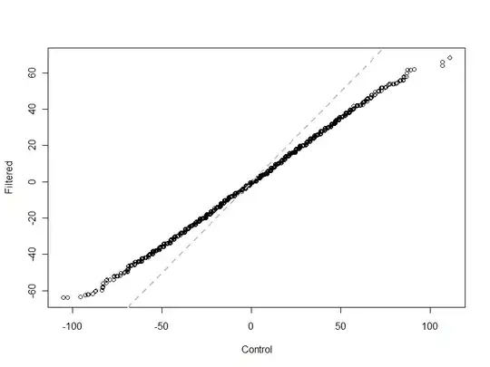
(The points were jittered slightly to resolve the thousands of overlaps: $B$ can have only integral values, after all.)

In this Q-Q plot, the control (on the horizontal coordinate) varies as expected: it's centered at 0 and stays generally between $-100$ and $100$. The statistic from the "filtered" dataset, using "bias removal," varies much less: only between about $-65$ and $65$. This is shown by the sharp departure between the simulated data (black circles) and the line $y=x$ (dashed gray).

In short, this effort to remove bias actually can create bias.

For some analyses, the bias introduced by this "bias removal" procedure will be small and wholly undetectable. Seeing the bias requires that $B$ and $A$ be correlated, probably strongly; and certain statistics will be more sensitive to it than others. But if nothing else, this simulation demonstrates that the "bias removal" procedure can create erroneous results.

A theoretical analysis of this effect would be difficult to carry out in most cases, I suspect. Simulations like this one can help determine the extent to which "bias removal" actually adds bias. But why go to all that effort when the sample is perfectly fine to begin with?