The data you describe here is often modeled as a Poisson process, i.e.
$Y \sim Po(\lambda t)$
where $Y$ is the number of goods produced in time $t$ and $\lambda$ is the rate of good production. The conjugate prior here is a Gamma distribution on $\lambda$, i.e. $\lambda \sim Ga(a,b)$, which results in a Gamma posterior, i.e. $\lambda \sim Ga(a+y,b+t)$.
Since you have two individuals, you can add subscripts, e.g. $Y_A \sim Po(\lambda_A t_A)$ and $Y_B \sim Po(\lambda_B t_B)$. I will make the assumption that the number of products produced by each worker are independent of the the number of products produced by the other worker (but this may not be true).
The conjugate prior for $\lambda_A,\lambda_B$ is independent Gamma distributions, i.e. $\lambda_A \sim Ga(a_A,b_A)$ and independently $\lambda_B\sim Ga(a_B,b_B)$. Then the posterior is independent Gamma distributions, i.e. $\lambda_A|y_A,y_B \sim Ga(a_A+y_A,b_A+t_A)$ and independently $\lambda_B|y_A,y_B \sim Ga(a_B+y_A,b_B+t_B)$.
In order to complete the analysis, you need to choose some values for $a_A,b_A,a_B,b_B$. If you have some prior knowledge, you should incorporate that here. For illustrative purposes, I will use $a_A=b_A=a_B=b_B=0$ which is an improper distribution but will have a proper posterior so long as $y_A>0$ and $y_B>0$. If you use these values, then your posteriors will look like the posteriors below.
curve(dgamma(x, 180, 100), 0, 4, col='red', lty=2,
      xlab=expression(lambda), ylab="Density")
curve(dgamma(x, 2, 1), add=TRUE)
legend("topright", c("Worker A", "Worker B"), col=c("black","red"), lty=1:2)
Notice that there is much more certainty about Worker B's production rate than there is about Worker A. This is due to the much longer time frame you have had to evaluate Worker B.
Now you are likely interested in the difference between these parameters, i.e. $\delta = \lambda_A-\lambda_B$ so that you can ask questions about how much better one worker is than the other. This is the difference of two gamma random variables and is discussed here. Instead of finding the analytical solution described there, I will take a simulation based approach, i.e. I will draw a bunch of values for $\lambda_A$ and $\lambda_B$ and take their difference. Then I can plot this or see what the probability is that it is greater than zero, i.e. my estimate of the probability that worker A is more productive than worker B.
lambdaA <- rgamma(1e5,2,1)
lambdaB <- rgamma(1e5,180,100)

delta <- lambdaA - lambdaB
mean(delta>0)
I find the estimated probability that work A is more productive than worker B is $\approx$0.46. The posterior of this difference is below.
hist(delta, 101, prob=TRUE, xlab=expression(delta), ylab="Density")
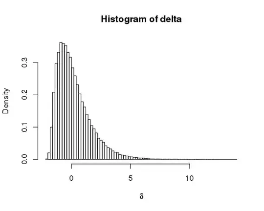
In addition to the 0.46 value (which is the area under the histogram to the right of 0), this figure provides the range of values for how much more productive worker A would be than worker B. Worker B could be as much as 5 goods per hour more productive down to ~2 goods per hour less productive.

