Examples of errors in MCMC algorithms

Question

I'm investigating a method for automatic checking of Markov chain Monte Carlo methods, and I would like some examples of mistakes that can occur when constructing or implementing such algorithms. Bonus points if the incorrect method was used in a published paper.

I'm particularly interested in cases where the error means that the chain has the incorrect invariant distribution, though other types of errors (e.g. chain not ergodic) would be of interest as well.

An example of such an error would be failing to output a value when Metropolis-Hastings rejects a proposed move.

Answer 1

Darren Wilkinson on his blog gives a detailed example of a common mistake in random walk Metropolis-Hastings. I recommend reading it in full, but here is the tl;dr version.

If the target distribution is positive (like Gamma distributions etc) in one dimension, it is tempting to reject proposals that have a negative value on that dimension straight away. The mistake is to throw away the proposals like they never happened and evaluate the Metropolis-Hastings (MH) acceptance ratio of the other ones only. This is a mistake because it amounts to using a non symmetric proposal density.

The author suggests to apply one of two fixes.

1. Count the "negatives" as failing acceptance (and lose a bit of efficiency).

2. Use the correct MH ratio in that case, which is

$$ \frac{\pi(x^*)}{\pi(x)} \frac{\Phi(x)}{\Phi(x^*)}, $$

where $\pi$ is the target density and $\Phi$ is the normalization constant of the truncated random walk proposal $\phi$, i.e. $\Phi(x) = \int_0^{\infty} \phi(y-x)dy$.

Answer 2

1. Marginal Likelihood and Harmonic mean estimator

The marginal likelihood is defined as the normalising constant of the posterior distribution

$$p({\bf x})=\int_{\Theta}p({\bf x}\vert\theta)p(\theta)d\theta.$$

The importance of this quantity comes from the role it plays in model comparison via Bayes factors.

Several methods have been proposed for approximating this quantity. Raftery et al. (2007) propose the Harmonic mean estimator, which quickly became popular due to its simplicity. The idea consists of using the relation

$$\dfrac{1}{p({\bf x})}=\int_{\Theta}\dfrac{p(\theta\vert{\bf x})}{p({\bf x}\vert\theta)}d\theta.$$

Therefore, if we have a sample from the posterior, say $(\theta_1,...,\theta_N)$, this quantity can be approximated by

$$\dfrac{1}{p({\bf x})}\approx\dfrac{1}{N}\sum_{j=1}^N \dfrac{1}{p({\bf x}\vert\theta_j)}.$$

This approximation is related to the concept of Importance Sampling.

By the law of large numbers, as discussed in Neal's blog, we have that this estimator is consistent. The problem is that the required $N$ for a good approximation can be huge. See Neal's blog or Robert's blog 1, 2, 3, 4 for some examples.

Alternatives

There are many alternatives for approximating $p({\bf x})$. Chopin and Robert (2008) present some Importance sampling-based methods.

2. Not running your MCMC sampler long enough (specially in the presence of multimodality)

Mendoza and Gutierrez-Peña (1999) deduce the reference prior/posterior for the ratio of two normal means and present an example of the inferences obtained with this model using a real data set. Using MCMC methods, they obtain a sample of size $2000$ of the posterior of the ratio of means $\varphi$ which is shown below

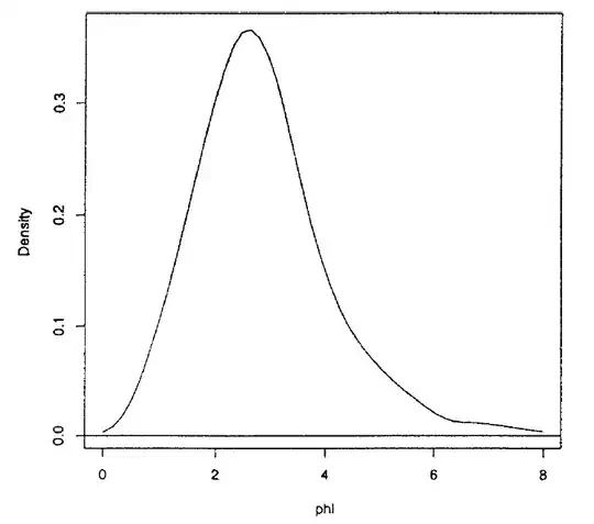
And obtain the HPD interval for $\varphi$ $(0.63,5.29)$. After an analysis of the expression of the posterior distribution, it is easy to see that it has a singularity at $0$ and the posterior should actually look like this (note the singularity at $0$)

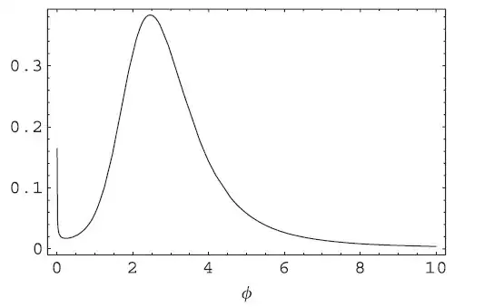
Which can only be detected if you run your MCMC sampler long enough or you use an adaptive method. The HPD obtained with one of these methods is $(0,7.25)$ as has already been reported. The length of the HPD interval is significantly increased which has important implications when its length is compared with frequentist/classical methods.

3. Some other issues such as assessing convergence, choice of starting values, poor behaviour of the chain can be found in this discussion by Gelman, Carlin and Neal.

4. Importance Sampling

A method for approximating an integral consists of multiplying the integrand by a density $g$, with the same support, that we can simulate from

$$I=\int f(x)dx = \int \dfrac{f(x)}{g(x)}g(x)dx.$$

Then, if we have a sample from $g$, $(x_1,...,x_N)$, we can approximate $I$ as follows

$$I\approx \dfrac{1}{N}\sum_{j=1}^N \dfrac{f(x_j)}{g(x_j)}.$$

A possible issue is that $g$ should have tails heavier/similar than/to $f$ or the required $N$ for a good approximation could be huge. See the following toy example in R.

# Integrating a Student's t with 1 d.f. using a normal importance function   
x1 = rnorm(10000000)   # N=10,000,000
mean(dt(x1,df=1)/dnorm(x1))

# Now using a Student's t with 2 d.f. function
x2 = rt(1000,df=2)
mean(dt(x2,df=1)/dt(x2,df=2))

Answer 3

A very clear case (connected with the marginal likelihood approximation mentioned in the first answer) where true convergence is the example of the problem of label switching in mixture models coupled with the use of Chib's (1995) estimator. As pointed out by Radford Neal (1999), if the MCMC chain does not converge correctly, in the sense that it does explore some of the mode of the target distribution, the Monte Carlo approximation of Chib fails to reach the right numerical value.