An activation function $h(x)$ with derivative $h_0
(x)$ is said to right (resp. left) saturate if
its limit as $x → ∞$ (resp. $x → −∞$) is zero. An activation
function is said to saturate (without qualification) if it both
left and right saturates.
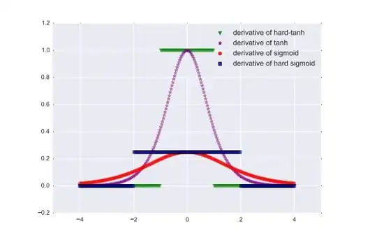
Most common activation functions used in recurrent networks
(for example, tanh and sigmoid) are saturating. In particular
they are soft saturating, meaning that they achieve saturation
only in the limit.
Let $c$ be a constant such that $x > c$ implies $h_0(x) = 0$ and left hard
saturates when $x < c$ implies $h_0(x) = 0, ∀x.$ We say that
h(·) hard saturates (without qualification) if it both left and
right hard saturates. An activation function that saturates but
achieves zero gradient only in the limit is said to soft saturate.
We can construct hard saturating versions of soft saturating
activation functions by taking a first-order Taylor expansion
about zero and clipping the results to an appropriate range.
For example, expanding tanh and sigmoid around 0, with
$x ≈ 0$, we obtain linearized functions $u_t$
and $u_s$ of tanh and
sigmoid respectively:
$sigmoid(x) ≈ u_s(x) = 0.25x + 0.5$
$tanh(x) ≈ u_t(x) = x$
Clipping the linear approximations result to,
$hard-sigmoid(x) = max(min(u_s(x), 1), 0)$
$hard-tanh(x) = max(min(u_t(x), 1), − 1)$
The motivation behind this construction is to introduce linear
behavior around zero to allow gradients to flow easily when
the unit is not saturated, while providing a crisp decision in
the saturated regime.
The ability of the hard-sigmoid and hard-tanh to make crisp
decisions comes at the cost of exactly 0 gradients in the
saturated regime. This can cause difficulties during training:
a small but not infinitesimal change of the pre-activation
(before the nonlinearity) may help to reduce the objective
function, but this will not be reflected in the gradient.
