6

I'd like help considering two different strategies in performing my regression.

Strategy 1:

model the output y as a linear combination of input variables x1 through x3:

fit = lm(y ~ x1 + x2 + x3)

Strategy 2:

model the output y with a linear relationship single input variable x1, and then model the residual of that through x2 etc:

firstFit = lm(y ~ x1)
firstResidual = y - predict(firstFit)
secondFit <- lm(firstResidual ~ x2 + 0) # Only one intercept
secondResidual = firstResidual - predict(secondFit)
thirdFit <- lm(secondResidual ~ x3 + 0) # Only one intercept

Questions:

  1. What are the differences between these two strategies?
  2. Can I expect that the "quality" of the coefficients in Strategy 1 to be uniform across X, and in Strategy 2 to not be?
  3. Strategy 1 seems generally the way to go, what would be a circumstance where Strategy 2 would be better?
  4. If I believe that the "truth" is that y is the output of a nested set of functions:
    y = f1(x1, f2(x2, f3(x3))),
    would Strategy 2 be an appropriate way to model the system?
kmace
  • 737
  • 4
  • 17
  • This situation is thoroughly explained--with examples, figures, and code--at https://stats.stackexchange.com/a/46508/919. The theory is described again at https://stats.stackexchange.com/a/113207/919. – whuber Aug 11 '17 at 13:51

1 Answers1

5

The second strategy is the same linear model, but with a different/inferior estimation procedure.


Let's look at the sequential approach more closely, with two covariates $X_1$ and $X_2$. After regressing $Y$ on $X_1$, we have:

$$\hat Y = b_0 + b_1X_1$$

Now, you want to regress the residuals on $X_2$. Thus, the model we are assuming is,

$$Y - \hat Y = \alpha_0 + \alpha_1 X_2 + \epsilon$$

Or equivalently,

\begin{align*} Y &= \hat Y + \alpha_0 + \alpha_1 X_2 + \epsilon \\ &= (b_0 + \alpha_0) + b_1 X_1 + \alpha_1 X_2 + \epsilon \end{align*}

It seems to me, that the sequential approach is more or less a roundabout way, to getting the same linear model, with a different estimation procedure.

  1. Strategy 1 $$Y = \beta_0 + \beta_1X_1 + \beta_2X_2 + \epsilon$$
  2. Strategy 2 $$Y = (b_0 + \alpha_0) + b_1 X_1 + \alpha_1 X_2 + \epsilon$$

Since the OLS estimators are the Best Linear Unbiased Estimators for normally distributed $\epsilon$, it's hard to imagine that the second approach could offer any improvement.


Simulations

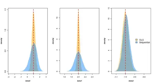
I simulated $n=100$ data points from the model $Y = 1 + 2X_1 - X_2 + \epsilon$, where $\epsilon \sim N(0, 1)$. Repeating the simulation $10,000$ times, we can consider sampling distributions for the OLS and sequential procedures.

enter image description here

The estimation of $\beta_3$ is comparable for both cases, but the OLS estimation procedure leads to more precise estimation of $\beta_0$ and $\beta_1$.

knrumsey
  • 5,943
  • 17
  • 40
  • 3
    +1 I'll just add that Strategy 2 is known as [Gram-Schmidt process](https://en.wikipedia.org/wiki/Gram%E2%80%93Schmidt_process) and generally avoided because of numeric instability. – juod Aug 11 '17 at 07:54
  • Note that those two approaches only return the same estimates if X_1 and X_2 do not share the same variance with Y. It would be nice to see a discussion of the same question in this general case. – jmb Dec 18 '19 at 15:34