For all $t\in 1,\dots,T$, suppose $x_t\in [0,1]$ is a draw from a distribution with unknown CDF $F:[0,1]\rightarrow [0,1]$. For future use, define $\tilde{x}\in [0,1]^T$ to be a vector containing $x_1,\dots,x_T$ sorted into increasing order.
Suppose further that we know that $F$ is strictly increasing and continuous, and so has full support and no mass points.
The usual estimate of $F$ is the empirical CDF: $$\hat{F}_T^{\mathrm{E}}(z)=\frac{1}{T}\sum_{t=1}^T{\mathbb{1}[x_t\le z]},$$ but this will neither be strictly increasing, nor continuous.
Now for $u,v\in [0,1]^T$, define $g_{u,v}:[0,1]\rightarrow [0,1]$ as the unique continuous, piecewise linear function with knot points at $0,u_1,\dots,u_T,1$ taking the values $0,v_1,\dots,v_T,1$, respectively.
Using this notation, we may define three other alternative estimators: $$\hat{F}_T^{\mathrm{L}}(y)=g_{\tilde{x},[0,\frac{1}{T},\frac{2}{T},\dots,\frac{T-1}{T}]}(y),$$ $$\hat{F}_T^{\mathrm{H}}(y)=g_{\tilde{x},[\frac{1}{T},\frac{2}{T},\dots,1]}(y),$$ $$\hat{F}_T^{\mathrm{M}}(y)=g_{\tilde{x},[\frac{1}{T+1},\frac{2}{T+1},\dots,\frac{T}{T+1}]}(y).$$ All three estimators are continuous, but only $\hat{F}_T^{\mathrm{M}}$ is strictly increasing.
Furthermore, it is easy to see that $\hat{F}_T^{\mathrm{L}}(y)\le\hat{F}_T^{\mathrm{E}}\le\hat{F}_T^{\mathrm{H}}$ and that $\hat{F}_T^{\mathrm{L}}(y)\le\hat{F}_T^{\mathrm{M}}\le\hat{F}_T^{\mathrm{H}}$.
Asymptotically, all four estimators are equivalent, but in finite samples, my hunch is that $\hat{F}_T^{\mathrm{M}}$ ought to perform better.
Can one give any justification for using $\hat{F}_T^{\mathrm{M}}$ beyond the fact it is strictly increasing and continuous? E.g. it the maximum likelihood estimator of $F$ when $F$ is drawn from some reasonable distribution? Or is there some connection to maximum entropy?
I am tagging this with bootstrap, as the $\hat{F}_T^{\mathrm{E}}$ and $\hat{F}_T^{\mathrm{L}}$ estimators are used in constructing bootstrap p-values from source test p-values, and I am contemplating doing the same with the $\hat{F}_T^{\mathrm{M}}$ estimator.
Edit: Suggestive evidence.
Suppose that $F(z)=z$, and that $T=1$. Then:
$${\hat{F}}_{1}^{\mathrm{E}}\left( z \right)\mathbb{= 1}\left\lbrack x \leq z \right\rbrack$$
$${\hat{F}}_{1}^{\mathrm{L}}\left( z \right) = \min\left\{ \frac{z}{x},1 \right\}$$
$${\hat{F}}_{1}^{\mathrm{H}}\left( z \right) = \max\left\{ 0,\frac{z - x}{1 - x} \right\}$$
$${\hat{F}}_{1}^{\mathrm{M}}\left( z \right) = \min\left\{ \frac{z}{2x},\frac{1}{2} \right\} + \max\left\{ 0,\frac{1}{2} - \frac{1 - z}{2\left( 1 - x \right)} \right\}$$
$$\mathbb{E}{\hat{F}}_{1}^{\mathrm{E}}\left( z \right) = \int_{z}^{1}{0\mathbb{d}x} + \int_{0}^{z}{1\mathbb{d}x} = z$$
$$\mathbb{E}{\hat{F}}_{1}^{\mathrm{L}}\left( z \right) = \int_{z}^{1}{\frac{z}{x}\mathbb{d}x} + \int_{0}^{z}{1\mathbb{d}x} = z - z\log z$$
$$\mathbb{E}{\hat{F}}_{1}^{\mathrm{H}}\left( z \right) = \int_{z}^{1}{0\mathbb{d}x} + \int_{0}^{z}{\frac{z - x}{1 - x}\mathbb{d}x} = z + \left( 1 - z \right)\log\left( 1 - z \right)$$
$$\mathbb{E}{\hat{F}}_{1}^{\mathrm{M}}\left( z \right) = \int_{z}^{1}{\frac{z}{2x}\mathbb{d}x} + \int_{0}^{z}{\left\lbrack 1 - \frac{1 - z}{2\left( 1 - x \right)} \right\rbrack\mathbb{d}x} = z + \frac{1}{2}\left( 1 - z \right)\log\left( 1 - z \right) - \frac{1}{2}z\log z$$
$$\mathbb{E}\left( {\hat{F}}_{1}^{\mathrm{E}}\left( z \right) - F(z) \right)^{2} = \int_{z}^{1}{\left( 0 - z \right)^{2}\mathbb{d}x} + \int_{0}^{z}{\left( 1 - z \right)^{2}\mathbb{d}x} = z\left( 1 - z \right)$$
$$\mathbb{E}\left( {\hat{F}}_{1}^{\mathrm{L}}\left( z \right) - F(z) \right)^{2} = \int_{z}^{1}{\left( \frac{z}{x} - z \right)^{2}\mathbb{d}x} + \int_{0}^{z}{\left( 1 - z \right)^{2}\mathbb{d}x} = 2z\left( 1 - z + z\log z \right)$$
$$\mathbb{E}\left( {\hat{F}}_{1}^{\mathrm{H}}\left( z \right) - F(z) \right)^{2} = \int_{z}^{1}{\left( 0 - z \right)^{2}\mathbb{d}x} + \int_{0}^{z}{\left( \frac{z - x}{1 - x} - z \right)^{2}\mathbb{d}x} = 2\left( 1 - z \right)\left( z + \left( 1 - z \right)\log\left( 1 - z \right) \right)$$
$$\mathbb{E}\left( {\hat{F}}_{1}^{\mathrm{M}}\left( z \right) - F(z) \right)^{2} = \int_{z}^{1}{\left( \frac{z}{2x} - z \right)^{2}\mathbb{d}x} + \int_{0}^{z}{\left( 1 - \frac{1 - z}{2\left( 1 - x \right)} - z \right)^{2}\mathbb{d}x} = z^{2}\log z + \left( 1 - z \right)^{2}\log\left( 1 - z \right) + \frac{3}{2}z\left( 1 - z \right)$$
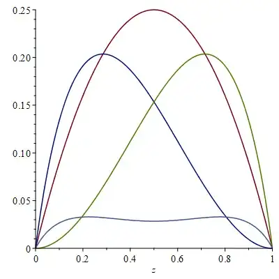
The figure below plots $\mathbb{E}\left( {\hat{F}}_{1}^{\mathrm{E}}\left( z \right) - F(z) \right)^{2}$ in red, $\mathbb{E}\left( {\hat{F}}_{1}^{\mathrm{L}}\left( z \right) - F(z) \right)^{2}$ in dark blue, $\mathbb{E}\left( {\hat{F}}_{1}^{\mathrm{H}}\left( z \right) - F(z) \right)^{2}$ in green and $\mathbb{E}\left( {\hat{F}}_{1}^{\mathrm{M}}\left( z \right) - F(z) \right)^{2}$ in light blue.
The $\mathrm{M}$ estimator has the lowest MSE despite its bias.
Ideally though, I would like to prove a result like this without making assumptions on what $F$ is. (Assumptions on the distribution from which $F$ is drawn are fine, providing they have full support on the class of distributions described. E.g. $F(z)=\frac{\int_0^z{(\exp{W(\tau)}+J(\tau))\mathbb{d}\tau}}{\int_0^1{(\exp{W(\tau)}+J(\tau))\mathbb{d}\tau}}$, where $W$ is standard Brownian motion and $J$ is a pure jump process with e.g. exponentially distributed jump sizes.)
