5

What methods are there to fit a model of the form $y=A\mathrm e^{Bx}+C\mathrm e^{Dx}+E$?

Here is the actual scientific data to be fitted: http://dl.dropbox.com/u/39499990/Ben%2C%20real%20data.xlsx

B should be in the range of -1 to -100.

D should be in the range of -100 to -500.

E is a constant.

This specific model is of interest as it is an accepted one in the scientific community for describing the biological proccess in hand- Inactivation of a voltage dependent calcium channel. (for reference see for example: A novel molecular inactivation determinant of voltage-gated CaV1.2 L-type Ca2+ channel. A Livneh, R Cohen, and D Atlas; Neuroscience, Jan 2006; 139(4): 1275-87. " The rate of inactivation was analyzed by a biexponential decay -A1exp(-t/Tao1)-A2exp(-t/Tao2)+C " )

Best would be a solution that I could implement in Excel, by the use of build-in functions or VBA code.

Glen_b
  • 257,508
  • 32
  • 553
  • 939
Michael Litvin
  • 285
  • 3
  • 7
  • Presumably the last "$e$" does not mean the same thing as the first two "$e$"s! Some more information about the data and your expectations about $B$ and $D$ would help, because in general fitting functions like this can be tricky. For an example (with a related function) please read the replies at http://stats.stackexchange.com/questions/7308/. – whuber May 19 '12 at 22:20
  • I'm working with Michael Litvin on this issue. Here is the actual scientific data to be fitted: http://dl.dropbox.com/u/39499990/Ben%2C%20real%20data.xlsx B should be in the range of 1-100. D should be in the range of 100-500. E is a contant, not e. – Ben May 21 '12 at 20:25
  • One would expect both $B$ and $D$ to be *negative*, @Ben, given that the data appear to have a negative second derivative. The sum of exponentials looks like it will be a poor fit. Could you disclose the reasons why this form of function is expected? Could you explain the nature of $x$ and $y$ so we can understand what functional forms would be likely and what kinds of errors to expect? – whuber May 21 '12 at 21:20
  • The plot looks much more like a rational function than anything involving exponentials. E.g., try $y = -52.5245 - 6.05282/(x - 0.364724)$. (This is not the best possible: the residuals have interesting structure.) – whuber May 21 '12 at 21:44
  • @whuber you're right, $B$ and $D$ should be negative. Edited the question. – Michael Litvin May 22 '12 at 17:51
  • Re The edit: I doubt that a sum of exponentials is the usual one describing these kinetics. More likely people use a rational expression in exponentials, not a sum. Could you provide a reference or link to an example? – whuber May 22 '12 at 19:23

3 Answers3

3

Best is not a solution in Excel -- spreadsheets are not a good environment for data analysis: http://www.burns-stat.com/pages/Tutor/spreadsheet_addiction.html

The 'nls' function in R would be one choice.

Patrick Burns
  • 1,037
  • 7
  • 6
3

I'll show you how to analyze your data with Mathematica. First I'll use your model as requested.

data = Import["Desktop/data.csv"];
y = NonlinearModelFit[data, 
  a Exp[b x] + c Exp[d x] + e, {a, b, c, d, e}, x];

Mathematica returns this error:

NonlinearModelFit::cvmit: Failed to converge to the requested accuracy or precision within 1000 iterations

This means that your model might not be ideal. Let's consider the data to see if we can come up with a better one. The log-plot of the negative of your series (so we can take the logarithm) shows a fairly polynomial curve:

Log-plot of raw data

(Generated using ListLogPlot[# {1, -1} & /@ data])

This suggests that instead of an exponential mixture, we should use a log-linear model:

$ \hat y = -\exp(a+bx+cx^2 + \dots)$

Let's try a cubic polynomial:

nlm = LinearModelFit[{#[[1]], Log[-#[[2]]]} & /@ data, {x, x^2, x^3}, x]

Mathematica returns 71.6838 - 391.293 x + 764.791 x^2 - 501.198 x^3

In other words,

$ \hat y = -\exp(71.6838 - 391.293 x + 764.791 x^2 - 501.198 x^3)$.

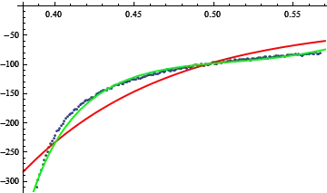
Here is a plot of the data, the mixture model (red), and the log-linear model (green):

Final result

(Generated using Show[{ListPlot@data, Plot[y[x], {x, 0.38, 0.57}, PlotStyle -> {Thick, Red}], Plot[-Exp@nlm@x, {x, .35, 0.6}, PlotStyle -> {Thick, Green}]}])

You can get an ever better fit with a quartic polynomial, but you get the idea. The residuals show structure, which means that the model has not squeezed all the information out of the data:

Residual of cubic polynomial

(Generated using ListPlot@nlm["FitResiduals"])

Fortunately, the order virtually disappears by the time you raise the order to six:

Residual of hexic polynomial

Emre
  • 2,564
  • 15
  • 22
  • Nice--but you are working too hard. See http://new.nutonian.com/download/. Use it to explore reasonable fits, then analyze them in greater detail with *Mathematica.* Incidentally, Mathematica *can* converge to a modest fit with the double-exponential formula: you need to supply better starting values, that's all. – whuber May 21 '12 at 22:10
  • @whuber: Thanks for the software suggestion. I got the double exponential to fit all right (you can see it in the plot), but the fit was not good enough in my opinion so I sought a better model. Did you find a better fit with the mixture model? – Emre May 21 '12 at 22:17
  • I found a good five-parameter fit as a rational function of $\exp(x)$ and $\exp(2 x)$. It suggests the second and third data points (from the left) are outliers (there's a hint of that in your last plot) and it slightly overestimates values for larger $x$. A case could be made for finding one fit for the most negative values of $y$ (less than $-300$, say) and another for the rest, but its merit depends on the scientific purposes of the fitting exercise, of which we unfortunately still remain ignorant. – whuber May 22 '12 at 14:24
1

Are you looking for methods or software to implement it? It looks like a typical nonlinear regression problem. In SAS this is implemented using proc nlin.

Michael R. Chernick
  • 39,640
  • 28
  • 74
  • 143