Poisson Binomial Distribution with Evenly Distributed Bernoulli Trial Probabilities

Question

Consider the Poisson binomial distribution with $n$ coins and coin probabilities ${1 \over n}, {2\over n}, \dots, {n-1 \over n}, 1$. Do we know an asymptotic for this distribution?

Le Cam's theorem says when the $p_i$ are small the distribution approaches Poisson($\mu)$, but the $p_i$ are not small here. We can even say it's not Poisson: by the Stein-Chen method applied by Barbour and Hall a lower bound on total variation distance between the Poisson($\mu$) and Poisson binomial distribution with coin probabilities $p_i$ is $$\frac{1}{32} \min (\frac{1}{\mu}, 1) \displaystyle\sum_{i=1}^n p_i^2$$ In our case $\mu$ and $\sum p_i^2$ are $\Theta(n)$ so this is $\Omega(1)$.

Note that the last coin doesn't do anything but shift the mean of the distribution, so it's probably easier just to eliminate it (since you'll subtract the mean back off when working out the asymptotics); you can always just stick its effect back in at the end. Incidentally it looks like in practice you should be able to use a normal approximation with fairly modest values of $n$, unless you need far tail probabilities. A continuity correction looks to be useful for the main bulk of the distribution. — Glen_b, Jun 22 '17 at 02:18

score 2 · Accepted Answer · answered May 04 '19 at 15:58

Intuitively, there's no problem because for each $k=1, 2, \ldots, n$ we may pair the variable of mean $k/n$ with that of mean $(n-k)/n$ (except possibly when $2k=n,$ which will not matter asymptotically). The sum of these variables has mean $1/2$ and (obviously) has no skewness. The variances of these sums are

$$\frac{k}{n}\left(1 - \frac{k}{n}\right) + \left(1 - \frac{k}{n}\right)\frac{k}{n} = 2\frac{k}{n}\left(1 - \frac{k}{n}\right)$$

which range from $2/n^2$ to $1/2.$ This range might give us pause, but asymptotically it causes no problems: when we standardize the sum (its mean is $\mu(n)=(1+n)/2$ and its variance is $\sigma^2(n)=(n^2-1)/(6n),$ both elementary computations) it converges fairly rapidly to a standard Normal distribution. The excess kurtosis is always negative (the tails are obviously limited in extent) but shrinks to zero.

A rigorous demonstration computes that the cumulant generating function of the standardized sum is $t^2/2 + O(n^{-1})O(t^4)$ which converges as $n$ grows large to the c.g.f. of the standard Normal distribution.

As a check, this R simulation generates 10,000 such sums for $n=20$ and visually compares their distribution to the Normal distribution with parameters $\mu(20),\sigma^2(20):$

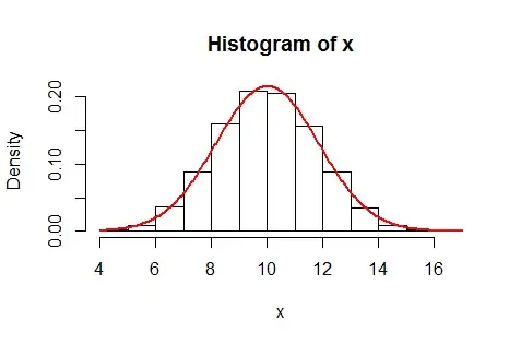
The red curve plots the corresponding theoretical probabilities. It is (already) an excellent fit.

n <- 20
n.sim <- 1e4
set.seed(17)

p <- (1:n)/n
x <- colSums(matrix(rbinom(n*n.sim, 1, p), nrow=n))

hist(x, freq=FALSE, breaks=min(x):max(x))
m <- sum(p)
v <- sum(p * (1-p))
curve(pnorm(x+1, m, sqrt(v)) - pnorm(x, m, sqrt(v)), col="Red", add=TRUE, lwd=2, n=301)

Poisson Binomial Distribution with Evenly Distributed Bernoulli Trial Probabilities

1 Answers1