This doesn't really have much to do with ROC curves. It is also true, as @FrankHarrell comments, that it is generally best not to use thresholds and classify observations at all. Having said that, the theoretical issue here is straightforward: The question of whether the threshold based on a predicted probability and a threshold based on a predictor value are equivalent is just the question of whether the mapping between them is one to one. If it is, then they are equivalent, and if not, not. I am less savvy with SVMs, so I will demonstrate this with logistic regression.
Here you can see that for every possible threshold defined on the predicted probabilities corresponds to exactly one possible threshold defined on the x-axis. That is because the logistic function here is a strictly monotonic (in this case increasing) function; that is, it is one to one.
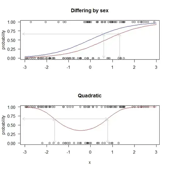
However, there are many ways in which the function that maps an x-value to a probability may not be one to one. Here are two easy examples: First, we have a case where the function that maps the x axis to a probability varies based on whether the patient is male or female. What we see is that a predicted probability of $.67$ corresponds to two different x-values, depending on the sex of the patient. Thus, there is no single x-value that corresponds to a given probability. Of course, given sex there still is a single x-value that corresponds to a given probability one to one, so the data could be stratified by sex and the physician would choose the appropriate threshold for each patient. But consider the second example below. In that case, no stratification is possible. If an x-axis threshold is preferred, it will have to be a more complicated rule.
The code I used to create these is below. The examples are coded in R, but the code is intended to be self-explanatory even for those who do not use R:
## the initial one to one function
set.seed(7197)                    # this makes the example exactly reproducible
x  = runif(100, min=-3, max=3)    # uniform x values in [-3, 3]
lo = 0 + 1*x                      # the true data generating process in ln odds
p  = exp(lo) / (1+exp(lo))        # ... converted to probabilities
y  = rbinom(100, size=1, prob=p)  # ... & used to generate Bernoulli trials

m1 = glm(y~x, family=binomial)    # a simple logistic regression model
summary(m1)$coefficients          # these are the fitted coefficients
#               Estimate Std. Error   z value     Pr(>|z|)
# (Intercept) -0.3605034  0.2532622 -1.423439 1.546088e-01
# x            1.0717952  0.2206656  4.857102 1.191161e-06

## the function differing by sex
set.seed(8575)
fem = sample(0:1, size=100, replace=TRUE)  # this generates women & men
lo3 = -.5 + 1*x + 1*fem
p3  = exp(lo3) / (1+exp(lo3))
y3  = rbinom(100, size=1, prob=p3)

m3 = glm(y~x+fem, family=binomial) # a multiple logistic regression model
summary(m3)$coefficients           # these are the fitted coefficients
#                Estimate Std. Error    z value     Pr(>|z|)
# (Intercept)  0.04557544  0.3622137  0.1258247 8.998707e-01
# x            1.10824172  0.2289450  4.8406467 1.294173e-06
# fem         -0.80493142  0.5185561 -1.5522553 1.206012e-01

## this is the quadratic version
set.seed(7197)
lo2 = 0 + 1*x + -.1*x^2            # now I added a squared function of x
p2  = exp(lo2) / (1+exp(lo2))
y2  = rbinom(100, size=1, prob=p2)

m2 = glm(y~x+I(x^2), family=binomial)  # a quadratic logistic regression model
summary(m2)$coefficients               # these are the fitted coefficients
#                Estimate Std. Error    z value     Pr(>|z|)
# (Intercept) -0.28945619  0.3171968 -0.9125444 3.614822e-01
# x            1.07197696  0.2239663  4.7863318 1.698572e-06
# I(x^2)      -0.05431788  0.1472379 -0.3689124 7.121930e-01

