How to incorporate uncertainty of actual historical data into forecast prediction intervals?

Question

I wonder how we can incorporate uncertainty of the actual historical data into forecast prediction intervals. In other words, we would have for example 95% range instead of the data points for historical data. Does any forecast method in Forecast package support this sort of uncertainty?

Answer 1

No, there is no such function in forecast, nor in any other R package that I am aware of.

The conceptually simplest way of going about this would be to take your uncertain time series and simulate within the bounds or with the distribution that you assume. Then, for each simulation, fit a model. Then, simulate from the predicted distributions. Finally, summarize all the simulated predictions.

This allows you to use whatever method you prefer for your forecasting: ETS, ARIMA, whatever. Plus, it includes model uncertainty. Your uncertain time series may look seasonal, but once you account for the uncertainty in your measurements, you may not be all that sure about it any more - and accounting for this uncertainty in this way will attenuate the seasonality in the forecast.

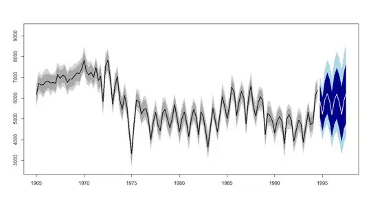
Here is a little example, using 100 simulations from the uncertain time series (normally distributed with standard deviation 300), forecasts using ETS, and another 100 simulations from each predictive distribution, along with 80% and 95% in-sample quantiles and out-of-sample prediction intervals:

Compare what we would get without accounting for the uncertainty in the historical data:

The prediction polygon (not the pointwise prediction intervals!) actually gets narrower in the top plot. This is a consequence of the fact alluded to above - many of the simulations result in non-seasonal models, because the uncertainty means we are not so sure about the seasonality any more:

> table(methods)
methods
ETS(A,N,A) ETS(M,A,A) ETS(M,N,A) 
        59          1         40

In a non-seasonal plot, I'd expect the prediction intervals to get wider in this way, of course.

library(forecast)

horizon <- 12
n.sims <- 1e2
n.sims.for.PIs <- 1e2
start.forecast <- c(1994,4)

set.seed(1)
sims.hist <- matrix(NA,nrow=n.sims,ncol=length(woolyrnq))
sims.fcst <- matrix(NA,nrow=n.sims*n.sims.for.PIs,ncol=horizon)

methods <- rep(NA,n.sims)
pb <- winProgressBar(max=n.sims)
for ( ii in 1:n.sims ) {
    setWinProgressBar(pb,ii,paste(ii,"of",n.sims))
    sims.hist[ii,] <- woolyrnq+rnorm(length(woolyrnq),0,300)
    model <- ets(ts(sims.hist[ii,],frequency=frequency(woolyrnq)))
    methods[ii] <- model$method
    for ( jj in 1:n.sims.for.PIs ) {
        sims.fcst[n.sims.for.PIs*(ii-1)+jj,] <- simulate.ets(model,nsim=horizon)
    }
}
close(pb)
table(methods)

conf <- c(0.8,0.95)
colors.hist <- c("darkgrey","lightgrey")
colors.fcst <- c("darkblue","lightblue")

ylim <- range(c(
    apply(sims.hist,2,quantile,prob=c((1-max(conf))/2,1-(1-max(conf))/2)),
    apply(sims.fcst,2,quantile,prob=c((1-max(conf))/2,1-(1-max(conf))/2))),
    forecast(woolyrnq,h=horizon,level=conf)$lower,
 forecast(woolyrnq,h=horizon,level=conf)$upper)

plot(ts(rep(1,length(woolyrnq)+horizon),start=start(woolyrnq),frequency=frequency(woolyrnq)),
    type="n",xlab="",ylab="",ylim=ylim)
for ( kk in seq_along(conf) ) {
    boundaries.hist <- apply(sims.hist,2,quantile,prob=c((1-rev(conf)[kk])/2,1-(1-rev(conf)[kk])/2))
    polygon(start(woolyrnq)[1]+(start(woolyrnq)[2]-2)/frequency(woolyrnq)+
            c(1:length(woolyrnq),length(woolyrnq):1)/frequency(woolyrnq),
        c(boundaries.hist[1,],rev(boundaries.hist[2,])),
        col=rev(colors.hist)[kk],border=NA)

    boundaries.fcst <- apply(sims.fcst,2,quantile,prob=c((1-rev(conf)[kk])/2,1-(1-rev(conf)[kk])/2))
    polygon(end(woolyrnq)[1]+(end(woolyrnq)[2]-1)/frequency(woolyrnq)+
            c(1:horizon,horizon:1)/frequency(woolyrnq),
        c(boundaries.fcst[1,],rev(boundaries.fcst[2,])),
        col=rev(colors.fcst)[kk],border=NA)
}
lines(woolyrnq,lwd=2)
lines(ts(colMeans(sims.fcst),start=start.forecast,frequency=frequency(woolyrnq)),lwd=2,col="white")

plot(forecast(woolyrnq,h=horizon,level=conf),ylim=ylim)