I found that, in examining the gender wage gap, there are cases where direct regression shows that men earn more than women with the same educational level (or qualification measured whatsoever) but men are more educated (or qualified) than women earning the same wage. Formally, if: $Y$ is wage, $E$ education and $G$ an indicator for being men: $Y=\alpha+\beta*E+\gamma*G$, and $E=\alpha^*+\beta^**Y+\gamma^**G$, we would have both $\gamma>0$ (an indicator of discrimination for women, paid less than men with the same educational level) and $\gamma^*>0$ (an indicator of discrimination for men, more educated than women with the same wage). I read that such paradox would not occurr if we could measure productivity without error (being education or measured qualification basically a proxy for it). However, what I'm interested in is (any variable could replace gender, wage and education) a fabricated simple numerical example (I was thinking at $2$ educational level and $2$ income levels, so to have a $2 \times 2 \times 2$ table) where this occurs. Alternatively, also how a mathematical demonstration that such situation could occurr would help.
References: Goldberger, Arthur. "Reverse Regression and Salary Discrimination," J. Human Res., 1984, 19(3), pp. 293-318
@ Gung: I read the paper from Greene. I'd say he doesn't believe in reverse regression. In fact, he shows that (equation 6): $c^*=\frac{(\bar{y}_f-\bar{y})*(1-R^2_{y,x,d})}{1-P}-c$, where $c$ and $c^*$ would be the discrimination coefficients (direct discrimination for $c<0$ and $c^*>0$, reverse discrimination for $c>0$ and $c^*<0$). This means that: $c^*>0 \iff c<\frac{(\bar{y}_f-\bar{y})*(1-R^2_{y,x,d})}{1-P}$. Assuming $c<0$ (direct discrimination found in direct regression), taking $k=-c(>0)$ and $k^*=-c^*$ (direct discrimination for $k^*<0$, reverse discrimination for $k^*>0$), it is: $k^*<0 \iff k> \frac{(\bar{y}-\bar{y}_f)*(1-R^2_{y,x,d})}{1-P}$.
Edited on June 12
Green concludes that "sign and magnitude" (of $c^*$) "may have nothing to do with discrimination".
Given $\bar{y}=\bar{y}_f*P+\bar{y}_m*(1-P)$, it is: $\bar{y}-\bar{y}_f=\bar{y}_f*(P-1)+\bar{y}_m*(1-P)=(\bar{y}_m-\bar{y}_f)*(1-P)$. Thus, $k^*<0 \iff k> \frac{(\bar{y}-\bar{y}_f)*(1-R^2_{y,x,d})}{1-P}=\frac{(\bar{y}_m-\bar{y}_f)*(1-P)*(1-R^2_{y,x,d})}{1-P}=(\bar{y}_m-\bar{y}_f)*(1-R^2_{y,x,d})$.
I'd say that $k$ reflects wage discrimination (in case employees consider qualification to be fully expressed by $E$), $1-R^2_{y,x,d}$ the part of variance of the wage depending on the error term $\epsilon$ (thus, unexplained) and $\bar{y}_m-\bar{y}_f$ the difference in wage, due to both discrimination and higher average education of men. Thus, $\bar{y}_m-\bar{y}_f>k$, and whether it will remain above $k$ even after multiplication by $(1-R^2_{y,x,d})$ depends on:
1) The difference in qualification between men and women (leading to higher $\bar{y}_m-\bar{y}_f$ independently of discrimination).
2) The variance of the error term, leading, in case of men and women earning the same salary, to lower educational level for women vs men (average $\epsilon$ higher for women in the direct regression), given the former have a lower global expected value than the latter).
Then, Greene studies the case where no discrimination was found in the 1st regression, showing that, with women earning less than men, a reverse discrimination would be found: this is due to the fact that, with all wage difference due to different qualification between men and women, in case of people earning the same wage, women have again an average value of the error term in the 1st regression higher than men, thus, a lower average educational level. Compared to the case with discrimination, $k=0$ implies that this will not be "compensated" by wage discrimination in direct regression, so there are no doubts about the sign of $k$.
Finally, he analyzes the case where men and women have the same average qualification, finding that discrimination in the two regressions would, in this case, agree in sign. This is because, with all wage difference due to discrimination, in case of people earning the same wage, women have not only (again) an average value of the error term in the 1st regression higher than men, but also a higher average educational level.
Compared to the case with different qualification between men and women, this time there is not a higher average qualification fo men, so men and women will "meet" at a point where women are more qualified, and the same discrimination as in direct regression will be found.
However, he says that the coefficient in reverse discrimination would be hard to interpret, because it would be just due to the one in direct regression multiplied by the $R^2$ of the regression of $Y$ on $X$, that should be "evidence against, not in support of, discrimination".
The point is that, with no error, we would measure the same discrimination as in direct regression. The higher the variance of the error, the higher the effect "women with higher $\epsilon$" than men, to decrease the estimated effect.
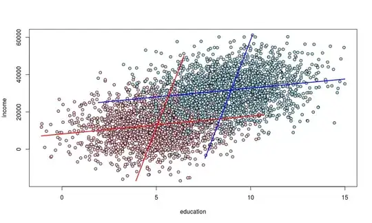
@ Martijn Weterings: It seems to me things are more easily understood if we notice that, with men having a higher educational level wrt women in average, if we compare men and women with the same wage, we are looking at a subset of the observations where women have higher $\epsilon$-values than men (even in absence of wage discrimination). If we had a problem of common support (the highest wage levels only available for men, the lowest one only for women), we could conclude that richest men would have an average $\epsilon$ higher than $0$, and the poorest women lower than $0$ to compensate for that. But, in a common support situation, it seems to me we would have a version of the Simpson's paradox: women would have a higher $\epsilon$ for each wage level, but, in the case of higher-wage groups (associated not only to being men - in case of discrimination, directly - and being more qualified, but also to higher $\epsilon$), we would find a higher number of men, and the other way round for lower-wage groups.

