It's a good question, because "different quantities" doesn't seem to be much of an explanation.
There are two important reasons to be wary of using $R^2$ to compare these models: it is too crude (it doesn't really assess goodness of fit) and it is going to be inappropriate for at least one of the models. This reply addresses that second issue.
Theoretical Treatment
$R^2$ compares the variance of the model residuals to the variance of the responses. Variance is a mean square additive deviation from a fit. As such, we may understand $R^2$ as comparing two models of the response $y$.
The "base" model is
$$y_i = \mu + \delta_i\tag{1}$$
where $\mu$ is a parameter (the theoretical mean response) and the $\delta_i$ are independent random "errors," each with zero mean and a common variance of $\tau^2$.
The linear regression model introduces the vectors $x_i$ as explanatory variables:
$$y_i = \beta_0 + x_i \beta + \varepsilon_i.\tag{2}$$
The number $\beta_0$ and the vector $\beta$ are the parameters (the intercept and the "slopes"). The $\varepsilon_i$ again are independent random errors, each with zero mean and common variance $\sigma^2$.
$R^2$ estimates the reduction in variance, $\tau^2-\sigma^2$, compared to the original variance $\tau^2$.
When you take logarithms and use least squares to fit the model, you implicitly are comparing a relationship of the form
$$\log(y_i) = \nu + \zeta_i\tag{1a}$$
to one of the form
$$\log(y_i) = \gamma_0 + x_i\gamma + \eta_i.\tag{2a}$$
These are just like models $(1)$ and $(2)$ but with log responses. They are not equivalent to the first two models, though. For instance, exponentiating both sides of $(2\text{a})$ would give
$$y_i = \exp(\log(y_i)) = \exp(\gamma_0 + x_i\gamma)\exp(\eta_i).$$
The error terms $\exp(\eta_i)$ now multiply the underlying relationship $y_i = \exp(\gamma_0 + x_i\gamma)$. Conseqently the variances of the responses are
$$\operatorname{Var}(y_i) = \exp(\gamma_0 + x_i\gamma)^2\operatorname{Var}(e^{\eta_i}).$$
The variances depend on the $x_i$. That's not model $(2)$, which supposes the variances are all equal to a constant $\sigma^2$.
Usually, only one of these sets of models can be a reasonable description of the data. Applying the second set $(1\text{a})$ and $(2\text{a})$ when the first set $(1)$ and $(2)$ is a good model, or the first when the second is good, amounts to working with a nonlinear, heteroscedastic dataset, which therefore ought to be fit poorly with a linear regression. When either of these situations is the case, we might expect the better model to exhibit the larger $R^2$. However, what about if neither is the case? Can we still expect the larger $R^2$ to help us identify the better model?
Analysis
In some sense this isn't a good question, because if neither model is appropriate, we ought to find a third model. However, the issue before us concerns the utility of $R^2$ in helping us make this determination. Moreover, many people think first about the shape of the relationship between $x$ and $y$--is it linear, is it logarithmic, is it something else--without being concerned about the characteristics of the regression errors $\varepsilon_i$ or $\eta_i$. Let us therefore consider a situation where our model gets the relationship right but is wrong about its error structure, or vice versa.
Such a model (which commonly occurs) is a least-squares fit to an exponential relationship,
$$y_i = \exp\left(\alpha_0 + x_i\alpha\right) + \theta_i.\tag{3}$$
Now the logarithm of $y$ is a linear function of $x$, as in $(2\text{a})$, but the error terms $\theta_i$ are additive, as in $(2)$. In such cases $R^2$ might mislead us into choosing the model with the wrong relationship between $x$ and $y$.
Here is an illustration of model $(3)$. There are $300$ observations for $x_i$ (a 1-vector equally distributed between $1.0$ and $1.6$). The left panel shows the original $(x,y)$ data while the right panel shows the $(x,\log(y))$ transformed data. The dashed red lines plot the true underlying relationship, while the solid blue lines show the least-squares fits. The data and the true relationship are the same in both panels: only the models and their fits differ.
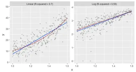
The fit to the log responses at the right clearly is good: it nearly coincides with the true relationship and both are linear. The fit to the original responses at the left clearly is worse: it is linear while the true relationship is exponential. Unfortunately, it has a notably larger value of $R^2$: $0.70$ compared to $0.56$. That's why we should not trust $R^2$ to lead us to the better model. That's why we should not be satisfied with the fit even when $R^2$ is "high" (and in many applications, a value of $0.70$ would be considered high indeed).
Incidentally, a better way to assess these models includes goodness of fit tests (which would indicate the superiority of the log model at the right) and diagnostic plots for stationarity of the residuals (which would highlight problems with both models). Such assessments would naturally lead one either to a weighted least-squares fit of $\log(y)$ or directly to model $(3)$ itself, which would have to be fit using maximum likelihood or nonlinear least squares methods.
