Looking for aberrations in time based data

Question

Looking at IO latency data for a storage array. When a drive is about to fail, one indication is an increase in the IO operations 'time to complete'. The array kindly provides this data in this format:

 Time                           Disk Channels
seconds   A      B      C      D      E      F      G      H      P      S
  0.017 5e98bd 64008b 62a559 68eb45 676ccf 5d3a86 46242b 62dd2e 6976c9 6da51f
  0.033 1e821c 1be769 1c372a 185134 19a2c2 21802c 2fa2ba 1d91c4 17b3ca 14cea6
  0.050  6638e  3a93b  4b19f  258aa  28b64  4d3ae  d92dc  32899  26a5b  1290d
  0.067   2df3   1c17   1f1b   180f   1291   1f05   5201   15f4   1856   10d8
  0.083    365    293    2b9    296    269    291    3c4    26f    2ae    25d
  0.100     ce     ae     94     aa     92     86     ce     81     9f     91
...

(time iterations go up to 2.00 seconds, counts are in hex).

The left column is the time the IO completes in, and the other columns are counts of IOs against a given spindle that completed in under that time.

When a drive is nearing failure, the 'tail' for that drive will get noticeably 'wider'... where most drives will have a small handful of IOs >0.2 seconds, failing drives can get lots of IOs over 0.2 seconds. Example :

Time Disk channels
seconds    A      B      C      D      E      F      G      H      P      S
...
0.200      4    52d      2      7      3      2      1      6      1      8
0.217      2    2a6      0      1      0      0      1      4      0      1
0.233      0    1a1      0      1      0      0      0      1      1      0
0.250      0     cb      0      1      0      0      1      1      0      1
0.267      0     73      0      0      0      0      0      0      0      0
0.283      0     44      0      0      0      0      0      0      0      0
0.300      0     2d      0      0      0      0      0      0      0      0
...

I could just look for more than 10 IOs over 0.2 seconds, but I was looking for a mathematical model that could identify the failures more precisely. My first thought was to calculate the variance of each column... any set of drives with a range of variances that was too broad, would flag the offender. However, this falsely flags drives behaving normally:

min variance is 0.0000437, max is 0.0001250.  <== a good set of drives
min variance is 0.0000758, max is 0.0000939.  <== a set with one bad drive.

I have thought about throwing away the first two rows of data (the largest counts by far), and seeing if the 'psudo-variance' gets cleaner, but tossing data in the trash doesn't make me happy. Any other ideas?

UPDATE: Here is my 'calculate' function (in python). I don't THINK there's a math error...:

def calculate(moment=1) :
    """loop through tiers, getting mean, and variance per drive in tier"""
    for tier in datadb.keys() :
        time_list = datadb[tier]['time_list']
        del(datadb[tier]['time_list'])
        for drive in sorted(datadb[tier].keys()) :
            summation = 0
            totalcount = 0
            for time, count in zip(time_list, datadb[tier][drive]) :
                summation += ( float(time) ** moment) * count
                totalcount += count
            calculated_moment = summation / totalcount
            moments.setdefault(tier, []).append( (drive,calculated_moment) )

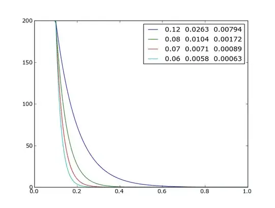
And here are 4 different runs, with the moment set to 1..4. For reference, tier 1 and 2 have no issues. Tier 12 and 14 have a 'long tail', and need to be replaced:

sum(t*n)/sum(n)
tier 1  min moment is 0.0198504, max is 0.0263216.  Worst drive is G
tier 2  min moment is 0.0254473, max is 0.0258425.  Worst drive is F
tier 12 min moment is 0.0229226, max is 0.0240188.  Worst drive is S
tier 16 min moment is 0.0195339, max is 0.0244102.  Worst drive is G

sum(t*t*n)/sum(n)
tier 1  min moment is 0.0004377, max is 0.0008179.  Worst drive is G
tier 2  min moment is 0.0007284, max is 0.0007539.  Worst drive is F
tier 12 min moment is 0.0006069, max is 0.0006693.  Worst drive is S
tier 16 min moment is 0.0004263, max is 0.0007183.  Worst drive is G

sum(t*t*t*n)/sum(n)
tier 1  min moment is 0.0000111, max is 0.0000295.  Worst drive is G
tier 2  min moment is 0.0000234, max is 0.0000251.  Worst drive is H
tier 12 min moment is 0.0000185, max is 0.0000222.  Worst drive is H
tier 16 min moment is 0.0000111, max is 0.0000256.  Worst drive is G

sum(t*t*t*t*n)/sum(n)
tier 1  min moment is 0.0000003, max is 0.0000013.  Worst drive is G
tier 2  min moment is 0.0000008, max is 0.0000020.  Worst drive is E
tier 12 min moment is 0.0000007, max is 0.0000015.  Worst drive is H
tier 16 min moment is 0.0000004, max is 0.0000046.  Worst drive is F

Answer 1

Calculating moments is often a good place to start when looking at the shape of the data. For example the normalized first moment Sum(t*n)/Sum(n) might be all you need here. That is, because you multiple by time, it gives more weight to the values that take longer time, and higher order moments would give even more weight to tail.

Sum(t*n)/Sum(n) is, of course, just the average time, but thinking in terms of moments gives the obvious next step of using higher order moments in determining the shape.

Here's a graph:

and the code to generate it:

import matplotlib.pyplot as plt
import numpy as np

t = np.linspace(0, 1., 200)

def f(a):
    f0 = np.exp(-a*(t-.1))
    i = np.searchsorted(t, .1)
    f0[:i] = 1
    return 200*f0

data = [f(a) for a in (10, 20, 30, 40)]


def process(t, f):
    moment0 = sum(f)
    moment1 = sum(t*f)
    moment2 = sum(t*t*f)
    moment3 = sum(t*t*t*f)

    v1 = moment1/moment0
    v2 = moment2/moment0
    v3 = moment3/moment0

    plt.plot(t, f)
    s = "%.2f  %.4f  %.5f" % (v1, v2, v3)
    return s

vals = []
for d in data:
    val = process(t, d)
    vals.append(val)
plt.legend(vals)

plt.show()

alternate:
An variant on this approach is that since you have a bunch of data, most of it from good disks, you could calculate your average distribution, and then look at the difference between this and each individual distribution, and then process this difference.

Final update:
OK, so maybe you need 4th order moments to get something really clear. Why? Consider some rough estimates of the 3rd order for the B drive, and compare the first elements contribution to the a point on the tail (6*16**5)*(.017**3)=31 to (4*16**1)*(.283**3)=1.5 There are a lot more points in the tail, but maybe 100s, not thousands, so maybe these don't add up well enough. If you use 4th order, these become (6*16**5)*(.017**4)=.52 and (4*16**1)*(.283**4)=.41, but again there are a lot more in the tail, so these should add up to something very distinct.

Answer 2

Looking at moments of the data may not be adequate because your observations, IO's/second, are not i.i.d; rather the process you are trying to model is Markovian i.e. the value at time $t$ depends on the value at time $t-1$.

One approach for modeling such data is to use a Hidden Markov Model (HMM). With an HMM you can model the data as being generated by given states e.g. normal, heavy, or failure, which can transition between each other with some given probability e.g. heavy is much more likely to transition to failure than normal is (this is the Markovian part). However, you cannot observe the underlying process (hence the hidden part); instead the hidden states emit observable variables, which in your case would be IOs/sec, with some probability, which for the sake of illustration could be Gaussian i.e. $IOs | failure \sim N(\mu_f, \sigma_f^2)$, where $\mu_f$ some value larger than the $\mu$ for the normal or heavy states.

In total, the parameters of an HMM are- the hidden states, the transition probabilities between states, the emission states, the emission probabilities, and the initial probabilities (what's the probability of starting the HMM at normal versus heavy versus failure?).

The simple Gaussian-HMM model alluded to above is taught in many introductory Machine Learning and Statistics courses. A simple Google search will lead you to practically implemented code in the language of your choice.

Of course the HMM can be extended ad infinitum; if you are interested in more flexible and complete modeling and you use R; check out the depmixS4 package.