Test to establish if there is a significant fluctuation in data?

Question

I'm not sure the best way to word this question, so excuse my ignorance.

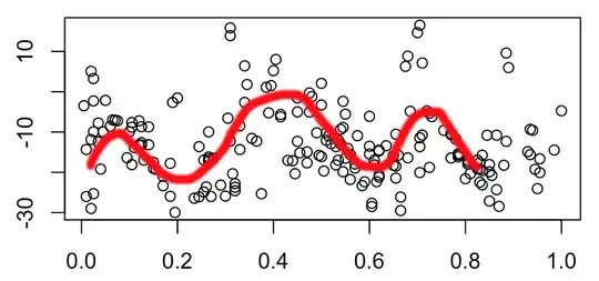
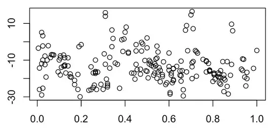
I'm working with some data that I am expecting to contain around three or four peaks or troughs:

I am pleased to note that the data appear to contain the wiggle I expected, which I have roughly superposed (hand-drawn) here:

I am able to make some predictions regarding the number of zero-crossings (three, or maybe four). I also am able to make some guesses at where I'd expect these to be. I'd like to keep as many of these assumptions free as possible, but can bring in these constraints to build a model if necessary.

I'm looking for a statistical test that will tell me if the data truly are 'wiggly', and ideally, would like to find the zero crossings. I recognise that this will involve playing with a few parameters (or perhaps fixing them according to my predictions), but am currently unsure where to begin in doing this.

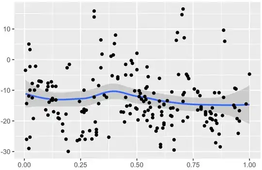
An attempt to fit a LOESS local regression results in the following:

I know that I could fiddle with the parameters until I make something fit, but I'd like to know the best way of doing this sensibly, and crucially, being able to state clearly that the pattern I'm seeing is real (albeit with a lot of noise). Perhaps this will involve building a model and then checking how well it fits the data.

Any suggestions for the sorts of techniques I could use would be appreciated. I understand that this is likely to involve some form of Time Series Analysis techniques, but due to the lack of an explicit periodicity, I'm not sure if that's entirely appropriate.

Here are the data in a form that can be imported into R:

dat <- structure(list(x = c(0.005, 0.01, 0.01, 0.02, 0.02, 0.02, 0.025, 
                      0.025, 0.025, 0.025, 0.035, 0.035, 0.04, 0.045, 0.05, 0.06, 0.065, 
                      0.07, 0.075, 0.095, 0.1, 0.105, 0.105, 0.105, 0.11, 0.12, 0.12, 
                      0.125, 0.125, 0.125, 0.13, 0.14, 0.14, 0.15, 0.15, 0.155, 0.17, 
                      0.17, 0.185, 0.185, 0.19, 0.195, 0.2, 0.235, 0.245, 0.245, 0.255, 
                      0.255, 0.26, 0.265, 0.265, 0.265, 0.265, 0.27, 0.275, 0.29, 0.3, 
                      0.305, 0.31, 0.31, 0.31, 0.315, 0.32, 0.32, 0.32, 0.33, 0.33, 
                      0.34, 0.34, 0.345, 0.355, 0.365, 0.375, 0.385, 0.39, 0.395, 0.4, 
                      0.405, 0.415, 0.415, 0.43, 0.44, 0.445, 0.45, 0.45, 0.45, 0.455, 
                      0.47, 0.47, 0.475, 0.475, 0.48, 0.49, 0.495, 0.5, 0.5, 0.5, 0.505, 
                      0.51, 0.51, 0.515, 0.52, 0.53, 0.53, 0.535, 0.535, 0.54, 0.54, 
                      0.545, 0.545, 0.545, 0.55, 0.55, 0.555, 0.56, 0.56, 0.57, 0.57, 
                      0.575, 0.585, 0.59, 0.6, 0.6, 0.6, 0.605, 0.605, 0.61, 0.61, 
                      0.615, 0.62, 0.62, 0.62, 0.62, 0.635, 0.65, 0.65, 0.655, 0.655, 
                      0.655, 0.66, 0.665, 0.665, 0.675, 0.68, 0.68, 0.685, 0.7, 0.705, 
                      0.705, 0.705, 0.705, 0.71, 0.71, 0.72, 0.725, 0.725, 0.73, 0.755, 
                      0.77, 0.77, 0.77, 0.78, 0.785, 0.785, 0.785, 0.8, 0.805, 0.805, 
                      0.805, 0.81, 0.825, 0.825, 0.83, 0.83, 0.83, 0.835, 0.835, 0.835, 
                      0.845, 0.85, 0.85, 0.85, 0.855, 0.865, 0.865, 0.87, 0.88, 0.885, 
                      0.885, 0.89, 0.93, 0.935, 0.935, 0.94, 0.945, 0.95, 0.955, 0.955, 
                      0.985, 1), y = c(-3.484848485, -14.33333333, -26.01010101, -11.88016529, 
                                       5.075757576, -28.98550725, -2.279957582, 3.26953748, -25.3030303, 
                                       -9.94531784, -12.45284186, -7.765616857, -19.21387791, -9.956709957, 
                                       -2.157738095, -8.596837945, -6.994849683, -7.070707071, -7.196969697, 
                                       -16.39118457, -9.924242424, -8.793706294, -7.662337662, -18.0952381, 
                                       -13.88888889, -13.19444444, -7.231404959, -8.683982684, -13.23076923, 
                                       -12.65477354, -16.99976625, -8.722222222, -13.16137566, -19.03053087, 
                                       -17.53472222, -19.26736881, -21.01449275, -23.33333333, -17.78390805, 
                                       -25.95818815, -2.660105548, -29.95495495, -1.550497866, -26.43467643, 
                                       -26.09302326, -13.63636364, -16.96521869, -24.88005997, -23.61078819, 
                                       -16.18135626, -17.21088435, -16.66666667, -9.964012596, -26, 
                                       -16.50219298, -23.1884058, -25.9, -6.566985646, -12.23958333, 
                                       15.85526316, 13.91304348, -20.35573123, -22.81329781, -23.71541502, 
                                       -24.57873934, -8.465608466, -14.35786436, 6.428571429, -2.651515152, 
                                       1.797385621, -11.58963585, -12.28475228, -25.31931932, 1.0998011, 
                                       -5.257936508, 1.520608243, 5.22875817, 8, -6.225895317, -5.663587749, 
                                       -17.04545455, -17.13842975, -20.34574468, -5, -12.31884058, -1.551226551, 
                                       -15.16312057, -14.92144026, -17.65005828, -0.310800311, -5.050505051, 
                                       -1.198801199, -10.19345238, -15.78947368, -16.11842105, -3.289473684, 
                                       2.083333333, -19.6827262, -12.06913435, -10.14739229, -10.995086, 
                                       -12.89146289, -13.63636364, -18.18181818, -12.0414673, -17.003367, 
                                       -9.339774557, -12.99302549, -19.86504279, -2.380952381, -8.873307544, 
                                       -16.51469098, -5.568181818, -14.08948195, -15.57002111, -21.78017241, 
                                       -18.9484127, -17.93478261, -10.91269841, -23.31492984, -22.35449735, 
                                       -15.45729403, -13.53383459, -6.111111111, -28.5, -27.69423559, 
                                       -17.00626959, -18.15942678, -22.33635929, -14.51133408, -20.6915564, 
                                       -14.69979296, -21.19883041, -13.40136054, -15.86466165, -18.25657895, 
                                       -18.48103372, -21.43438572, -10.53846154, -15.75833333, -26.14583333, 
                                       -29.49002217, 6.297117517, -16.40977444, 8.829365079, -4.861111111, 
                                       14.66303966, -20.06514165, -13.63636364, -11.44661408, 16.51515152, 
                                       -10.76388889, 7.126322751, -4.783549784, -18.79002359, -5.370985604, 
                                       -6.186868687, -9.588675214, -10.67725753, -10.35196687, -16.44736842, 
                                       -11.76201373, -15.72617946, -16.15516871, -15.3968254, -21.6, 
                                       -17.96831956, -17.02792299, -17.5, -20.34090909, -19.16076845, 
                                       -16.99083862, -22.4627451, -17.586727, -19.24242424, -23.11827957, 
                                       -19.58064516, -15.74898785, -10.80586081, -18.06375443, -27.13316096, 
                                       -19.87394958, -20.77922078, -10.79633056, -24.30992808, -28.45564516, 
                                       -18.24229692, -12.32492997, 9.598930481, 5.980861244, -14.87414188, 
                                       -15.6213705, -9.329798515, -9.565217391, -19.25465839, -24.06204906, 
                                       -20.07407407, -16.66666667, -14.47596533, -4.73172988)), .Names = c("x", 
                                                                                                           "y"), class = "data.frame", row.names = c(NA, -200L))

I see little evidence of zero-crossings in your example data. (Did you notice that there are no zero-crossings in the Loess smooth? Its confidence envelope never even comes near zero.) About the only way to obtain a good answer--apart from having an enormous dataset--will be to posit a specific parametric model for the data. Do you have such a model in mind? — whuber, Apr 20 '17 at 15:18
Testing implies a model. Do you have a candidate data generating model in mind? If not, this problem isn't well posed. — nth, Apr 22 '17 at 17:55
If you are looking for a "wiggle", do you mean zero crossings of the curve or its derivatives? (e.g. curvature sign changes) — GeoMatt22, Apr 22 '17 at 20:56
You could perhaps try something like your LOESS fit, but using cross-validation to explore generalization error as a function of the smoothing level (then, e.g. if this shows a well-defined optimum, you can assess how stable that is, similar to a "standard-error" on the parameter)? — GeoMatt22, Apr 23 '17 at 05:46
Expanding on whuber and Glen_b's comments: When you say "expecting to contain around three or four peaks or troughs", is this based on some underlying model (perhaps conceptual) of the underlying data-generating process? There is no fully general answer to your question as posed (aside from "it depends"). — GeoMatt22, Apr 23 '17 at 08:37

score 0 · Accepted Answer · 2017-04-23T05:21:09.603

Here's a solution using polynomial equations to fit the data. It's a python code but gets things done.

Loading required packages and data

import matplotlib.pyplot as plt
import pandas as pd
import numpy as np
from scipy.stats import linregress

#getting data into a dataframe
d=pd.DataFrame({'x':[0.005, 0.01, 0.01, 0.02, 0.02, 0.02, 0.025, 
      0.025, 0.025, 0.025, 0.035, 0.035, 0.04, 0.045, 0.05, 0.06, 0.065, 
      0.07, 0.075, 0.095, 0.1, 0.105, 0.105, 0.105, 0.11, 0.12, 0.12, 
      0.125, 0.125, 0.125, 0.13, 0.14, 0.14, 0.15, 0.15, 0.155, 0.17, 
      0.17, 0.185, 0.185, 0.19, 0.195, 0.2, 0.235, 0.245, 0.245, 0.255, 
      0.255, 0.26, 0.265, 0.265, 0.265, 0.265, 0.27, 0.275, 0.29, 0.3, 
      0.305, 0.31, 0.31, 0.31, 0.315, 0.32, 0.32, 0.32, 0.33, 0.33, 
      0.34, 0.34, 0.345, 0.355, 0.365, 0.375, 0.385, 0.39, 0.395, 0.4, 
      0.405, 0.415, 0.415, 0.43, 0.44, 0.445, 0.45, 0.45, 0.45, 0.455, 
      0.47, 0.47, 0.475, 0.475, 0.48, 0.49, 0.495, 0.5, 0.5, 0.5, 0.505, 
      0.51, 0.51, 0.515, 0.52, 0.53, 0.53, 0.535, 0.535, 0.54, 0.54, 
      0.545, 0.545, 0.545, 0.55, 0.55, 0.555, 0.56, 0.56, 0.57, 0.57, 
      0.575, 0.585, 0.59, 0.6, 0.6, 0.6, 0.605, 0.605, 0.61, 0.61, 
      0.615, 0.62, 0.62, 0.62, 0.62, 0.635, 0.65, 0.65, 0.655, 0.655, 
      0.655, 0.66, 0.665, 0.665, 0.675, 0.68, 0.68, 0.685, 0.7, 0.705, 
      0.705, 0.705, 0.705, 0.71, 0.71, 0.72, 0.725, 0.725, 0.73, 0.755, 
      0.77, 0.77, 0.77, 0.78, 0.785, 0.785, 0.785, 0.8, 0.805, 0.805, 
      0.805, 0.81, 0.825, 0.825, 0.83, 0.83, 0.83, 0.835, 0.835, 0.835, 
      0.845, 0.85, 0.85, 0.85, 0.855, 0.865, 0.865, 0.87, 0.88, 0.885, 
      0.885, 0.89, 0.93, 0.935, 0.935, 0.94, 0.945, 0.95, 0.955, 0.955, 
                      0.985, 1],
'y':[-3.484848485, -14.33333333, -26.01010101, -11.88016529, 
       5.075757576, -28.98550725, -2.279957582, 3.26953748, -25.3030303, 
       -9.94531784, -12.45284186, -7.765616857, -19.21387791, -9.956709957, 
       -2.157738095, -8.596837945, -6.994849683, -7.070707071, -7.196969697, 
       -16.39118457, -9.924242424, -8.793706294, -7.662337662, -18.0952381, 
       -13.88888889, -13.19444444, -7.231404959, -8.683982684, -13.23076923, 
       -12.65477354, -16.99976625, -8.722222222, -13.16137566, -19.03053087, 
       -17.53472222, -19.26736881, -21.01449275, -23.33333333, -17.78390805, 
       -25.95818815, -2.660105548, -29.95495495, -1.550497866, -26.43467643, 
       -26.09302326, -13.63636364, -16.96521869, -24.88005997, -23.61078819, 
       -16.18135626, -17.21088435, -16.66666667, -9.964012596, -26, 
       -16.50219298, -23.1884058, -25.9, -6.566985646, -12.23958333, 
       15.85526316, 13.91304348, -20.35573123, -22.81329781, -23.71541502, 
       -24.57873934, -8.465608466, -14.35786436, 6.428571429, -2.651515152, 
       1.797385621, -11.58963585, -12.28475228, -25.31931932, 1.0998011, 
       -5.257936508, 1.520608243, 5.22875817, 8, -6.225895317, -5.663587749, 
       -17.04545455, -17.13842975, -20.34574468, -5, -12.31884058, -1.551226551, 
       -15.16312057, -14.92144026, -17.65005828, -0.310800311, -5.050505051, 
       -1.198801199, -10.19345238, -15.78947368, -16.11842105, -3.289473684, 
       2.083333333, -19.6827262, -12.06913435, -10.14739229, -10.995086, 
       -12.89146289, -13.63636364, -18.18181818, -12.0414673, -17.003367, 
       -9.339774557, -12.99302549, -19.86504279, -2.380952381, -8.873307544, 
       -16.51469098, -5.568181818, -14.08948195, -15.57002111, -21.78017241, 
       -18.9484127, -17.93478261, -10.91269841, -23.31492984, -22.35449735, 
       -15.45729403, -13.53383459, -6.111111111, -28.5, -27.69423559, 
       -17.00626959, -18.15942678, -22.33635929, -14.51133408, -20.6915564, 
       -14.69979296, -21.19883041, -13.40136054, -15.86466165, -18.25657895, 
       -18.48103372, -21.43438572, -10.53846154, -15.75833333, -26.14583333, 
       -29.49002217, 6.297117517, -16.40977444, 8.829365079, -4.861111111, 
       14.66303966, -20.06514165, -13.63636364, -11.44661408, 16.51515152, 
       -10.76388889, 7.126322751, -4.783549784, -18.79002359, -5.370985604, 
       -6.186868687, -9.588675214, -10.67725753, -10.35196687, -16.44736842, 
       -11.76201373, -15.72617946, -16.15516871, -15.3968254, -21.6, 
       -17.96831956, -17.02792299, -17.5, -20.34090909, -19.16076845, 
       -16.99083862, -22.4627451, -17.586727, -19.24242424, -23.11827957, 
       -19.58064516, -15.74898785, -10.80586081, -18.06375443, -27.13316096, 
       -19.87394958, -20.77922078, -10.79633056, -24.30992808, -28.45564516, 
       -18.24229692, -12.32492997, 9.598930481, 5.980861244, -14.87414188, 
       -15.6213705, -9.329798515, -9.565217391, -19.25465839, -24.06204906, 
       -20.07407407, -16.66666667, -14.47596533, -4.73172988]})

Fitting

This chunk of code fits the given x and y data to polynomial equations ranging in degree from 1 to 8.

ns=range(1,9,1)
ax=plt.subplot(111)
d.plot.scatter(x='x',y='y',ax=ax)
metrics=pd.DataFrame(index=ns,columns=['r','standard error'])
for n in ns:
    fit = np.polyfit(d['x'], d['y'], n) 
    yp = np.poly1d(fit)
    _,_,r,_,e = linregress(yp(x), d['y'])
    metrics.loc[n,'r']=r
    metrics.loc[n,'standard error']=e    
    ax.plot(x, yp(x), '-',color=plt.get_cmap('Reds')(n/float(max(ns))),lw='3')
ax.legend(['degree=%d' % n for n in ns],bbox_to_anchor=(1.4, 1))

metrics.index.name='degree'
metrics.plot()

Results

Polynomial of degree 7 onwards the fluctuations (peaks and valleys) are correctly identified by the fitting model.

Increase in regression coefficient (between $y$ and $y_{pred}$) and Decrease in standard error of fitting proves that it is indeed a better fit of the given data.

$Decrease in standard error of fitting and increase in regression coefficient (between $y$ and $y_{pred}$)$

Cross validation

To check whether the the results were due to over-fitting, I used 10-fold cross validation. The oscillations are captured better as the degree of polynomial is increased (>7).

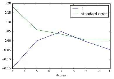
Interestingly, however, the metrics i.e. r and standard deviation show a saturation.

Code:

from sklearn.preprocessing import PolynomialFeatures
from sklearn.linear_model import LinearRegression
from sklearn.pipeline import Pipeline
from sklearn.model_selection import cross_val_predict

ax=plt.subplot(111)
d.plot.scatter(x='x',y='y',ax=ax,color='w')
ns=range(3,12,2)
metrics=pd.DataFrame(index=ns,columns=['r','standard error'])
for n in ns:
    lr = Pipeline([('poly', PolynomialFeatures(degree=n)),
                  ('linear', LinearRegression(fit_intercept=False))])
    X=d['x'].as_matrix().reshape(1,-1).T
    y=d['y'].as_matrix()
    yp=cross_val_predict(lr, X,y, cv=10)
    _,_,r,_,e = linregress(yp, d['y'])
    metrics.loc[n,'r']=r
    metrics.loc[n,'standard error']=e    
    ax.plot(d['x'], yp, '-',color=plt.get_cmap('jet')((n-min(ns))/float(max(ns)-min(ns))),lw='3')
    ax.set_ylim([-40,20])
ax.legend(['degree=%d' % n for n in ns],bbox_to_anchor=(1.4, 1))

metrics.index.name='degree'
metrics.plot()

I am not sure the reason why the metrics of fitting saturate but the oscillations are better captured at degree>7. But overall, polynomial of degree 11 seems to be the best fit here.

Not sure if polynomials are a reliable approach here: even with little data (that has no real "wiggles") a high order polynomial will tend to give oscillations! (see [here](https://en.wikipedia.org/wiki/Runge%27s_phenomenon) and also [here](https://stats.stackexchange.com/questions/233414/why-are-there-large-coefficents-for-higher-order-polynomial)) — GeoMatt22, Apr 22 '17 at 20:59
While @GeoMatt22 is not sure if polynomials are a reliable approach, I am not sure the reason why they wouldn't be a reliable approach. `high order polynomial will tend to give oscillations!` (`Runge's phenomenon`) is the very reason why I used them to test for the oscillations. Correct me if I am wrong but `high order polynomial will tend to give oscillations!` would be a context dependent advantage or disadvantage. — , Apr 23 '17 at 02:56
Did you try cross-validation? Your plot seems to be just a function of the data misfit (with "test set" = train set). Note that an $N+1$ degree polynomial will *exactly* fit the $N$ data points. — GeoMatt22, Apr 23 '17 at 03:29
@GeoMatt22 Please see the updated section : `Cross validation`. Its interesting that now polynomials with degree>7 are best capturing the oscillations. However `r` and `standard error` do not change. — , Apr 23 '17 at 05:24

Test to establish if there is a significant fluctuation in data?

1 Answers1

Loading required packages and data

Fitting

Results

Cross validation