5

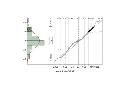
I am running a linear mixed model with 4 fixed factors and 1 random factor. The response variable is %growth and it has negative values (some of my animals shrunk). The problem I'm having is the residuals are not normally distributed according to the shapiro wilk test. The histogram seems like a normal distribution, but the normal quantile plot has an s-curve. In looking this up, I've found this curve labeled fat tail, short tail, and long tail.

I have tried transforms (log, sqrt, cube root) but nothing seems to make it normal (log doesn't work at all bc of the negative values). My next step would be to try a generalize linear mixed model, but I use JMP and it doesn't offer that functionality yet. Do I have any options aside from learning R?

My n is 304, and I have heard that normality matters less as sample size increases, but I don't think 304 is very large.

Edit: I have heard that % growth is not a great response variable for ANOVA, and that perhaps I should do an ANCOVA with final length as the response variable, and initial length as a covariate. However, this also gives me an s-curve and non-normal residuals.

residual histogram and normal quantile plot

Nathan Haag
  • 141
  • 7
  • 304 is not huge, but it is large enough for small violations from normality to hopefully be unproblematic. Sadly, "hopefully" is not such a scientifically useful term. I'd be surprised if the problem disappears with a mixed model. The model of final length as a response variable seems risky to me, as you will likely need to interact all your other variables with initial length. Can JMP compute bootstrapped p-values? That would seem to me to be the nice solution here. – Tim Feb 28 '17 at 01:04
  • Have you tried using log(final length) as response variable and log(initial length) as a covariate or offset? – EdM Feb 28 '17 at 01:24
  • @Tim I will look into bootstrapping today and get back to you. You are right about the interactions with initial length - I tried it and it caused a loss of degrees of freedom for all my fixed effects. – Nathan Haag Feb 28 '17 at 13:47
  • @EdM All of the interaction terms would likely cause a loss of DF, but I will try the log x log ANCOVA – Nathan Haag Feb 28 '17 at 13:47
  • @Tim I'm not sure how I would do bootstrapping in JMP (I've never done bootstrapping at all). My search resulted in a bootstrap function that is only available in JMP Pro which I do not have, and it is performed on one-way analysis. I think even if I had the enhanced program, that option would not work as I have 4 factors plus the random factor. – Nathan Haag Feb 28 '17 at 16:21
  • @EdM Using log x log with all the other factors results in a loss of DF. Adding log(initial) as a covariate without any interactions leaves me with a similar s-curve – Nathan Haag Feb 28 '17 at 16:24
  • Am I correct that your data consist of initial and final length measurements, along with 4 fixed factor values at the initial time, for each of 304 individuals? – EdM Feb 28 '17 at 18:48
  • @EdM I have initial and final length (along with width and height but their data behave similarly). The 4 fixed factors are 3 experimental treatments and the remaining fixed factor is species. I am working with two very similar species - When I remove species from my model, I can see that one of the two species is driving this s-curve. And in addition to those four factors, I also have blocking (randomized complete block) as a random factor. – Nathan Haag Feb 28 '17 at 19:46
  • Maybe the kind people at SAS will give you a trial of pro? I am doubtful that changing the functional form of your model (e.g., transformations, interactions) are going to solve this problem. (The whole idea of transforming data to create normal residuals is something that appears in all textbooks, but in my experience rarely works once you have real-world data with more than a few observations.) – Tim Feb 28 '17 at 21:15
  • Does JMP support SAS macro language? If so, then it would be easy to introduce one of the widely available bootstrap macros. Your plot shows clear nonlinearity. To me, it looks like a succession or series of diffusion curves. Being linear, ANOVA is definitely not appropriate. My suggestion would be to employ a robust, nonparametric method such as quantile regression. There's a paper on *boosting additive quantile regression* by Hyndman, et al, that describes one approach to this. – Mike Hunter Feb 28 '17 at 22:15
  • Thanks @DJohnson. i'm not sure about the macro, but I think it might. I'll look for the paper and get back to you. – Nathan Haag Mar 01 '17 at 00:50
  • I neglected to mention that, once the quantiles are in place, any probabilistic distribution can be fit to them, including Cauchy, Levy stable, whatever. Estimating a tail index would facilitate the choice. – Mike Hunter Mar 01 '17 at 15:36

3 Answers3

5

Growth rates must be distributed as some variation of the Cauchy distribution. I have written a series of papers on this. The Cauchy distribution has no mean so it has no variance or covariance. You can find my author page at https://papers.ssrn.com/sol3/cf_dev/AbsByAuth.cfm?per_id=1541471

Start with the paper titled "The distribution of returns," and then switch to the paper on Bayesian methods. Generally speaking, there is no admissible non-Bayesian solution though in specific cases there is a maximum likelihood solution that can be used if a null hypothesis method is required. The Bayesian likelihood function is always minimally sufficient.

You can communicate with me through the address on the author page. Because there is no variance or covariance, ANOVA and ANCOVA are impossible.

EDIT With regard to the comments:

1)If I say it's Cauchy, and therefore rule out ANOVA and ANCOVA, what are my options?

Bayesian regression is still available. Your likelihood function would be $$\frac{1}{\pi}\frac{\sigma}{\sigma^2+(y-\beta_0-\beta_1x_1-b_2x_2\dots\beta_nx_n)^2}$$

The meaning is very different from OLS, though. OLS is from a convergent process, such as water going down a drain. This can be conceived as a double pendulum problem, and as such has limited predictive capapcity. For example, if you had $y|x$ you could think of $x$ as the upper pendulum and $y$ as the lower pendulum attached to the top pendulum. So, while $y$ is affected by the movement of $x$ it does not mean they are even moving in the same direction with a positive correlation. A pendulum swinging to the left could cause the other pendulum from momentum to swing to the right.

There is a tight linkage between the double pendulum problem, which is the first real observed problem in chaos theory, and regression in this case.

The proper interpretation is that, for example, if $y=1.1x$ then 50% of the time $y$ will be greater than $1.1x$ and fifty percent of the time it will be less than $1.1x$. You may be able to make stronger statements if there are other properties in your system, such as non-negativity.

2) I've read that Cauchy is problematic if residuals are almost normal.

This does not matter. You can find, or even construct, cases where the Cauchy distribution is indistinguishable from a normal distribution. Generally speaking there is no admissible non-Bayesian solution for most standard problems. This is a problem for someone trained only in Frequentist methods, but is not a problem per se. If a null hypothesis is required by the nature of the problem, then the only close solution would be quantile regression or Theil's regression. The problem with either is that, in the above equation, $x_1$ and $x_2$ are not independent, but they are also not correlated.

The question is not Gaussian versus Cauchy by some empirical test, but which should I have from theory. A certain percentage of the time, data drawn from a pure normal distribution will falsify a test of normality through chance alone. While it is sometimes true we do not know the likelihood function and must test for it, sometimes we do. This is a case where we do.

3) Is this really growth rate if I only have initial and final length?

Yes that is a growth rate, it is just a growth rate with limited observations per creature.

Not asked

Is there anything similar to anova or ancova? The answer is "it is unclear." If you will notice there is only one scale parameter in the likelihood and this does not depend on the number of variables. The scale parameter is a composite of the separate scale parameters, but it is not clear that there is any way to take advantage of this.
Dave Harris
  • 6,957
  • 13
  • 21
  • I've sent you a message, but for the benefit of others: 1)If I say it's Cauchy, and therefore rule out ANOVA and ANCOVA, what are my options? 2) I've read that Cauchy is problematic if residuals are almost normal. 3) Is this really growth rate if I only have initial and final length? – Nathan Haag Feb 28 '17 at 16:26
  • 1
    You can't claim that all growth rates are from Cauchy. OP didn't even explain what growth rates are in question here. For instance, stable distributions have been tried on financial and economic data, there were a lot of academic papers on the subj. Yet, almost nobody applies stable distributions to these series anymore in the industry. They don't seem to work really – Aksakal Feb 06 '18 at 14:34
  • @Aksakal actually I can claim that. I understand your concern. In raw form, all growth rates or rates of returns must be a deformation of the Cauchy distribution, except for single period discount bonds, some specific cases for other bonds and cash-for-stock mergers. There is a missing ingredient in the older work. I wrote a book with a mathematician covering the expanse of methods of estimation and inference for distributions with heavy tails. It ranged from inference with the sign test to estimation using characteristic functions. – Dave Harris Feb 07 '18 at 01:16
  • @Aksakal what neither of us realized was how fragile these tools were to their assumptions, or where the inferences may not mean what is intended. We pulled the book from electronic availability subsequently. What triggered this was that I build a model to replace Black-Scholes that neither depends upon the underlying distribution nor the existence of a first moment as well as a parametric version and then tested it empirically. My goal was to test it using Pearson and Neyman's Frequentist methods, Fisher's Likelihoodist methods and Bayesian methods. – Dave Harris Feb 07 '18 at 01:20
  • @Aksakal The MLE doesn't have a closed form solution and I honestly have no clue how to perform a computable numerical estimate, but I decided I would estimate it by treating it as a MAP estimator with a flat prior. What surprised me was that the Frequentist solution did not match the Bayesian with roughly fifty million observations. – Dave Harris Feb 07 '18 at 01:22
  • @Aksakal I realized that the problem could be converted from an analytic problem to a geometry problem and with the population of data from the CRSP universe I could figure out what was going on by matching the geometry to the analytic solutions. The Bayesian matched and the Frequentist overestimated returns by 2% and underestimated risk by 4%. What I didn't realize at the time was that there does not exist an admissible non-Bayesian estimator. I also didn't realize there does not exist an unbiased estimator for the parameters. – Dave Harris Feb 07 '18 at 01:24
  • @Aksakal, while there are multiple issues involved, the two primary issues have to do with sufficiency and with truncation. There doesn't exist a point estimator that is sufficient. While this doesn't really matter for inference, it does for projection. The second issue is truncation. Truncation has a large impact on estimation. The mean of the log estimator is the median of the raw data, which is 2% off the actual location of $\mu$. – Dave Harris Feb 07 '18 at 01:29
  • @Aksakal I tried using the same tools everyone else was using and it failed for me too. In fact, the distribution of returns is a mixture of four core distributions plus a fifth type of distribution. There is also another process present that I haven't documented by which I realized was in the data. The reason you can say that growth in raw form is Cauchy distributed is that there is an existing statistical theorem that says it is and that this is true for any error term structure centered on zero with finite non-zero variance. – Dave Harris Feb 07 '18 at 01:36
  • @Aksakal This is also true for any AR(n) model as shown later by Rao. – Dave Harris Feb 07 '18 at 01:40
  • @DaveHarris, I read your (I think it was yours) excellent book on stable distributions, and attended a seminar with your presentation. I'm not denying that it's an interesting idea, and tried it myself on stock return series. The problem's that with equity returns there seem to be different distributions at different sampling frequencies. This doesn't fit the stable distribution idea. So, the high frequency series seem to have fat tails, but when you slow down the sampling the tails thin out. Even at high frequencies the fat tails don't seem to be Cauchy fat, but maybe student t level fat. – Aksakal Feb 07 '18 at 01:53
  • @DaveHarris, I won't claim that there are no Cauchy growth series, there could be some. Also, there are other ways to get fat tails e.g. exponentiating fat tailed distributions such as Student t. Suppose, that your log returns are t distributed, then the price series have very fat tails, and moments won't exist. These won't be stable distributions though. I think that certain financial series have this property, which makes their risk management "interesting." – Aksakal Feb 07 '18 at 01:59
4

Your Q-Q plot doesn't look like it has a fat tail. I'll show you how a fat tail looks like: enter image description here

Your tail is like a Victoria Secret's model compared to the above. I wish some of my model residuals had tails like yours has.

serv-inc
  • 273
  • 1
  • 2
  • 10
Aksakal
  • 55,939
  • 5
  • 90
  • 176
1

It seems that bootstrapping, as suggested by @Tim in comments, might be a good way to proceed. Even if your statistical software doesn't directly support bootstrapping it's not to hard to roll your own. For example, say you have all data for each individual in a single row (species; 3 treatment types; starting and ending length, width, and height; block ID) and you have 304 rows. You set up an index vector of length 304, and for each bootstrap fill it with a random sample with replacement from the integers from 1 to 304. You then take those indexed rows from your full data set for 304 rows total (with some original rows omitted, some taken once, and others 2 or more times). Then do your analysis and store the regression coefficients. Do this 999 times. For each regression coefficient, average the 999 results; then put its values for the 999 repetitions in rank order; the 25th and 975th in order set the 95% confidence limits. Unless your analysis depends heavily on having a balanced design, this should suffice.

This will not work if there is an underlying Cauchy problem, but I'm not convinced that you have this problem with your data set. The Cauchy problem comes from trying to take a ratio of 2 random variables in which you run a risk of dividing by zero or by numbers close to zero. Although this can be a serious issue in the types of economic time series addressed by @DaveHarris in the documents linked from his answer, in your case the lengths, widths and heights are all positive and far from zero so you don't seem to be in that situation. Raw differences between start and finish, or logs of start/finish ratios, should be sufficiently well behaved that you can analyze your data with the bootstrap, which is a well respected way to deal with your type of situation when you can't count on normal distributions of the data of interest.

EdM
  • 57,766
  • 7
  • 66
  • 187
  • This is a little over my head, but it seems promising...I'll see what I can do. – Nathan Haag Mar 01 '17 at 01:25
  • If you are at some type of academic institution, look into what local statistical support might be available. Also ask around for people who use R; this is very straightforward in R. If you intend to do a lot of projects requiring statistical analysis, consider devoting the time to getting up the initially steep learning curve in R; I did so a dozen years ago and am very glad I did. – EdM Mar 01 '17 at 01:48
  • I'm meeting with my R-literate lab mates today - they're suggesting glmm. If that doesn't work, I have the option to pay a small fee for someone from the stats department to do it. I still want to try this bootstrapping method - I found an add-in for jmp that does sampling with replacement, so I'll try that. I know that I have to learn R eventually, but I'm a PhD student and I'm trying to finish before I run out of money. – Nathan Haag Mar 01 '17 at 13:52
  • If you have R-literate labmates they should also be able to help you with the `boot` package in R, which essentially does what I outlined in the first paragraph of my answer. You just write a wrapper function that takes your complete data set and an index vector, and then returns the values of interest (regression coefficients here) for each bootstap sample. Then `boot()` does the resampling and `boot.ci()` returns several types of (empirical) confidence intervals. – EdM Mar 01 '17 at 15:06
  • Also, if one of your 2 species seems to have qualitatively different behavior from the other in terms of these residuals, it might make sense to analyze them separately. – EdM Mar 01 '17 at 15:08
  • I'm giving bootstrapping a quick try - but I have a quick question: what do I report, and how would I interpret the results? – Nathan Haag Mar 02 '17 at 21:01
  • You use the confidence intervals for regression coefficients among the bootstrap samples, instead of the confidence intervals you would have determined from the usual linear regression, for evaluating statistical significance. You probably should also report the values of the regression coefficients from the usual linear regression alongside their averages among the bootstrap samples so readers can compare them. – EdM Mar 03 '17 at 00:33