2

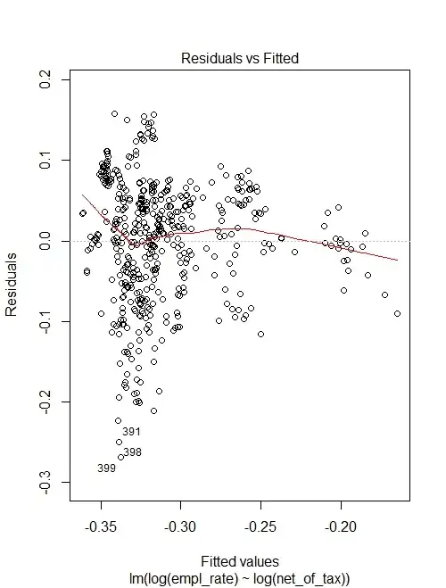
I am performing a simple linear regression with the lm() function to make statements about the association between the two variables. But I am not sure if my regression estimates and the t-test are correct due to the violations of assumptions (homoscedasticity and normal distribution of the error term)

My regression model looks as follows: log(employment rate) = a + e * log(net-of-tax), because I want to interpret the estimate as elasticity.

reg_test = lm(formula = log(empl_rate) ~ log(net_of_tax), data = dat)

plot(reg_test,1)

plot(reg_test,1)

The summary output looks like:

> summary(reg_test)

Call:
lm(formula = log(empl_rate) ~ log(net_of_tax), data = dat)

Residuals:
     Min       1Q   Median       3Q      Max 
-0.26905 -0.04372  0.00933  0.05167  0.15835 

Coefficients:
                 Estimate Std. Error t value Pr(>|t|)    
(Intercept)     -0.385486   0.007953  -48.47   <2e-16 ***
log(net_of_tax) -0.085839   0.008276  -10.37   <2e-16 ***
---
Signif. codes:  0 ‘***’ 0.001 ‘**’ 0.01 ‘*’ 0.05 ‘.’ 0.1 ‘ ’ 1
Residual standard error: 0.07481 on 477 degrees of freedom
Multiple R-squared:  0.184, Adjusted R-squared:  0.1823 
F-statistic: 107.6 on 1 and 477 DF,  p-value: < 2.2e-16

Am I correct in assuming that:

  • since heteroskedasticity does not bias the coefficient estimates it is possible to relax the assumption and just adjust the incorrect standard errors (e.g., using HC1), and
  • because of the large sample size, the error terms can deviate from normality?
gung - Reinstate Monica
  • 132,789
  • 81
  • 357
  • 650
Kaizen502
  • 29
  • 1
  • @subhashc.davar I am concluding the presence of heteroskedasticity because of the Fanning pattern in residuals versus fitted values plot. Even before the log-transformation there was a similar pattern. – Kaizen502 Dec 21 '16 at 17:16
  • The variable employment rate (OECD) is defined as a measure of the extent to which available labor resources (people available to work) are being used. They are calculated as the ratio of the employed to the working age population. And the net-of-tax is calculated using the participation tax rate – Kaizen502 Dec 21 '16 at 17:20
  • Heteroskedasticity looks obvious from the plot. Is the qq plot done without transformation? The qq plot looks fairly normal with some departure in the tails. – Michael R. Chernick Dec 21 '16 at 20:51
  • @MichaelChernick The qq-plot before transformation looks similar. Does this mean that the coefficient estimates are okay? – Kaizen502 Dec 21 '16 at 21:09
  • 2
    There is a better plot provided by R for looking for heteroscedasticity. It is the Scale-Location plot. Note that visual impression is not always a guide when you have denser regions at one end as they will inevitably be more dispersed. – mdewey Dec 22 '16 at 15:26
  • As you mentioned, the parameter estimates will be unbiased, the only thing that will be suspect is any inference you do on these coefficients (t-test, z-test etc). – bdeonovic Dec 22 '16 at 16:37
  • You should augment the OP with a scale-location plot, and look at some good advice here: http://stats.stackexchange.com/questions/147119/best-way-to-deal-with-heteroscedasticity – kjetil b halvorsen Dec 22 '16 at 19:51
  • @mdewey The scale-location plot also suggests heteroscedasticity and the p-value of the Breusch-Pagan test is < 0.05 – Kaizen502 Dec 23 '16 at 09:17

0 Answers0