This reply describes two good solutions, a permutation test and a Student t-test, and compares and contrasts them.
Michael Lew recommends a permutation test. This is good advice: such a test is conceptually simple and makes few assumptions. It interprets the null hypothesis as meaning it makes no difference which sample a value is from, because both samples are drawn from the same distribution. (Notice that this adds an unstated but common assumption; namely, that the distribution with mean $\mu_1$ has exactly the same shape as that with mean $\mu_2$.)
Because this dataset is so small--only 20 numbers are involved in two samples of 10 each--no simulation is needed to carry out the permutation test: we can directly obtain all $\binom{20}{10} = 184756$ distinct ways in which $10$ of the values can be drawn from all $20$ numbers. In each case we can compare the mean of the $10$ values (taken to represent possible values of $x$ under the null hypothesis) to the mean of the $10$ values that remain (i.e., the values of $y$): this is a natural statistic for comparing two means.
Here is a working R example:
x <- c(5,3,2,2,3,3,1,4,5,5)       # One sample
y <- c(4,3,1,3,5,2,2,3,5,3)       # The other sample

# Construct a test statistic
sum.all <- sum(c(x,y))
n.y <- length(y)
test.statistic <- function(u) mean(u) - (sum.all - sum(u)) / n.y

# Apply it to all possible ways in which x could have occurred.
perms <- combn(c(x,y), length(x))
p <- apply(perms, 2, test.statistic)

# Display the sample distribution of the test statistic.
hist(p)
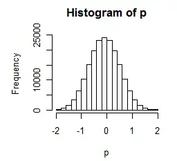
To use this histogram, note that the value of the test statistic for the actual observations is 0.2:
> test.statistic(x)
[1] 0.2
It is apparent in the histogram that many of the permutation results are larger in size than 0.2. We will quantify this in a moment, but at this point it is clear that the difference is relatively small.
It is worth noticing that the test statistic can only have a value in the range $[-2,2]$ in multiples of $0.2$: its sampling distribution is discrete.
> table(p)
p
   -2  -1.8  -1.6  -1.4  -1.2    -1  -0.8  -0.6  -0.4  -0.2     0
   35   154   560  1502  3316  6320 10356 15192 19679 23164 24200
  0.2   0.4   0.6   0.8     1   1.2   1.4   1.6   1.8     2
23164 19679 15192 10356  6320  3316  1502   560   154    35
(The numbers running -2 -1.8 ... 2 are the values of $p$ and beneath them are the numbers of times each occurs.)
We find, easily enough, that (a) 86.9% of the values are equal to or exceed the observed test statistic in size:
> length(p[abs(p) >= abs(test.statistic(x))]) / length(p)
[1] 0.8690164
and (b) 61.8% of the values strictly exceed the observed test statistic in size:
length(p[abs(p) > abs(test.statistic(x))]) / length(p)
[1] 0.6182641
There is little basis to choose one of these figures over the other; we might indeed just split the difference and take their average, equal to 0.744. This tells us that randomly dividing the 20 data values into two groups of 10 each, to simulate conditions under the null hypothesis, produces a greater mean difference either 87%, 62%, or 74% of the time, depending on how you wish to interpret "greater." These large results indicate the difference that has been observed could be attributed to chance alone: there is no basis for inferring the null hypothesis is false.
Anyone carrying out the calculations shown here would likely wait a few seconds for them to complete. They would not be practicable for larger datasets: in such cases there are just two many possible ways that sample $x$ could have occurred among all the numbers. That's why, when the two groups look similar and do not present a terribly skewed distribution, we often look first to a Student T test. This test is an approximation to the permutation test. It is intended to produce a comparable result while circumventing the large number of calculations needed to run the permutation test.
First we check that the t-test results may be applicable to these data:
> require("moments") # For skewness()
> sd(x)
[1] 1.418136
> sd(y)
[1] 1.286684
> skewness(x)
[1] -0.06406292
> skewness(y)
[1] 0.1385547
The two groups have comparable standard deviations and low skewnesses. Although they are small in size (10 numbers each), they are not too small. The t-test should therefore work well. Let's apply it:
> t.test(x,y, var.equal=TRUE, alternative="two.sided")

        Two Sample t-test

data:  x and y
t = 0.3303, df = 18, p-value = 0.745
alternative hypothesis: true difference in means is not equal to 0
95 percent confidence interval:
 -1.072171  1.472171
sample estimates:
mean of x mean of y
      3.3       3.1
The output is instantaneous, because little calculation is needed. As we saw before, the means differ by $3.3-3.1 = 0.2$. The p-value of 0.745 is remarkably close to the permutation test's result of 0.744 (q.v.).