Comparing t-SNE solutions using their Kullback-Leibler divergences

Question

I am trying to optimize the perplexity parameter of t-SNE in order to better understand the degree of separability of various data sets. Kullback-Leibler divergences of t-SNE solutions are directly comparable between runs when perplexity remains fixed as mentioned in the author's FAQ:

if you use the same data and perplexity, you can compare the Kullback-Leibler divergences that t-SNE reports. It is perfectly fine to run t-SNE ten times, and select the solution with the lowest KL divergence

Link here

My question is whether it's appropriate and useful to directly compare the KL divergences between runs but using different perplexities. I would then just select the solution with the lowest KL divergence

this comment to another question mentions:

tSNE has a theoretical optimum perplexity that minimizes the KL divergence between your data in its original and projected dimensions

Is comparing KL between runs with different perplexities a good way to find that "theoretical optimum perplexity?"

Answer 1

Unfortunately, no; comparing the optimality of a perplexity parameter through the correspond $KL(P||Q)$ divergence is not a valid approach. As I explained in this question: "The perplexity parameter increases monotonically with the variance of the Gaussian used to calculate the distances/probabilities $P$. Therefore as you increase the perplexity parameter as a whole you will get smaller distances in absolute terms and subsequent KL-divergence values." This is described in detail in the original 2008 JMLR paper of Visualizing Data using $t$-SNE by Van der Maaten and Hinton.

You can easily see this programmatically with a toy dataset too. Say for example you want to use $t$-SNE for the famous iris dataset and you try different perplexities eg. $10, 20, 30, 40$. What would be emperical distribution of the scores? Well, we are lazy so let's get the computer do the job for us and run the Rtsne routine with a few ($50$) different starting values and see what we get: (Note: I use the Barnes-Hut implementation of $t$-SNE (van der Maaten, 2014) but the behaviour is the same.)

library(Rtsne)
REPS =  50; # Number of random starts

per10 <- sapply(1:REPS, function(u) {set.seed(u); 
       Rtsne(iris, perplexity = 10, check_duplicates= FALSE)}, simplify = FALSE)
per20 <- sapply(1:REPS, function(u) {set.seed(u); 
       Rtsne(iris, perplexity = 20, check_duplicates= FALSE)}, simplify = FALSE)
per30 <- sapply(1:REPS, function(u) {set.seed(u); 
       Rtsne(iris, perplexity = 30, check_duplicates= FALSE)}, simplify = FALSE)
per40 <- sapply(1:REPS, function(u) {set.seed(u); 
       Rtsne(iris, perplexity = 40, check_duplicates= FALSE)}, simplify = FALSE)

costs <- c( sapply(per10, function(u) min(u$itercosts)), 
            sapply(per20, function(u) min(u$itercosts)),
            sapply(per30, function(u) min(u$itercosts)), 
            sapply(per40, function(u) min(u$itercosts)))
perplexities <- c( rep(10,REPS), rep(20,REPS), rep(30,REPS), rep(40,REPS))

plot(density(costs[perplexities == 10]), xlim= c(0,0.3), ylim=c(0,250), lwd= 2,
     main='KL scores from difference perplexities on the same dataset'); grid()
lines(density(costs[perplexities == 20]), col='red', lwd= 2); 
lines(density(costs[perplexities == 30]), col='blue', lwd= 2)
lines(density(costs[perplexities == 40]), col='magenta', lwd= 2);
legend('topright', col=c('black','red','blue','magenta'), 
       c('perp.  = 10', 'perp.  = 20', 'perp.  = 30','perp.  = 40'), lwd = 2)

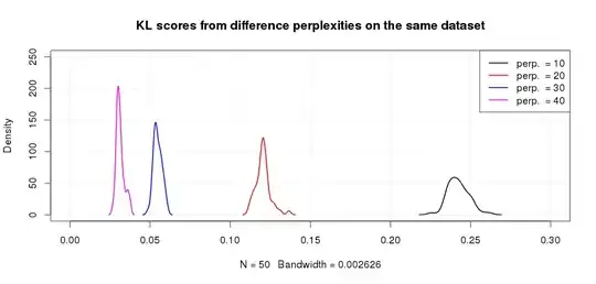
Looking at the picture it is clear that the smaller perplexity values correspond to higher $KL$ scores as expected based on the reading of the original paper above. Using the $KL$ scores to pick the optimal perplexity is not very helpful. You can still use it to pick the optimal run for a given solution though!