2

Let's say I have two signals $x_1$ and $x_2$, each having $N$ samples, i.e.:

$$ x_1 = \{ x_{11}, x_{12}, ..., x_{1N} \} $$ $$ x_2 = \{ x_{21}, x_{22}, ..., x_{2N} \} $$

The signals are both zero-mean. (Each signal's mean has already been subtracted from all of that signal's elements.)

Since the signals are both zero-mean, their moments and central moments are equal.

How can I calculate central moments of the joint probability density functions of $x_1$ and $x_2$?

In other words: How can I calculate $E[x_{1}^p x_{2}^q]$ for all positive integer values of $p$ and $q$?

I know how to compute $E[x_{1}^p x_{2}^q]$ when $p = q = 1$, but that's about it. I don't know how to do the calculation for larger values of $p$ and/or $q$.

The signals $x_1$ and $x_2$ are NOT statistically independent. If this were the case, it would be easy to compute as, for statistically independent signals: $E[x_{1}^p x_{2}^q] = E[x_{1}^p] E[x_{2}^q]$. This is not what I want.

Thank you very much for your help.

PS: Even the formulae which can be used to calculate/approximate these central moments (for finite samples) would be helpful, as I haven't been able to find them yet. It doesn't matter if there aren't any ready-to-use out-of-the-box Matlab functions, I'll then take care of coding the formulae myself.

UPDATE

When talking about statistical independence, does $E[x_{1}^p x_{2}^q]$ mean the first (central) moment of $x_1$ to the power of $p$, times $x_2$ to the power of $q$???

If this is the case, an example would be:

$$ x_1 = \sin(x)$$ $$ x_2 = \cos(x)$$

$E[x^2 y^3]$ is the first central moment of $\sin(x)^2 \cos(x)^3$, which is the mean of $\sin(x)^2 \cos(x)^3$ [for finite samples]

Can someone please verify this?

Thank you.

Macro
  • 40,561
  • 8
  • 143
  • 148
Rachel
  • 571
  • 2
  • 7
  • 17
  • **Something's not quite right here:** normally, people understand expressions like $E[X^p]$ to be *expectations* of *powers,* but you state explicitly this is not a power. Furthermore, $E[X_1^p, X_2^q]$ does not have any conventional sense. Do you seek the expectation of the *vector*-valued expression $(X_1^p, X_2^q)$ or do you want the $(p,q)$ moment, which is the expectation of the *product* $X_1^p X_2^q$? Finally, it appears you want these moments as *sample statistics,* but for what purpose? There are many possible estimators for any given moment; choosing one depends on its purpose. – whuber Mar 06 '12 at 21:44
  • @whuber You're right - the power part was a mistake, I apologise. I'd in fact edited the question seconds before I saw your comment. I actually need these to check whether two signals are statistically independent to each other. If so, E[x1^p x2^q] would be equal to E[x1^p] * E[x2^q]. I am already estimating E[x1^p] and E[x2^q] for all four central moments, but am stuck on the joint ones. Thank you for your help. – Rachel Mar 06 '12 at 22:19
  • See also [this related and very similar question](http://dsp.stackexchange.com/q/1579/235) on dsp.SE – Dilip Sarwate Mar 06 '12 at 22:27
  • @DilipSarwate I was actually the one who posted that question. It is related, but it's not the same. – Rachel Mar 06 '12 at 22:30
  • I know that you are the same one who posted on dsp.SE. Your question does not make much sense here either. – Dilip Sarwate Mar 06 '12 at 22:35
  • @DilipSarwate If you do not understand any part of the question, please tell me and I will update it. Other than that, it is a very crucial point for Independent Component Analysis. – Rachel Mar 06 '12 at 22:41
  • Rachel, your question as clarified by your comments *does* make sense. The attempt to state it in terms of higher-order multivariate moments introduces some inconsequential details: one does not usually use such moments to assess independence. You might attract more constructive responses by broadening your question: why not ask people how one goes about deciding whether two signals look independent? Tell us a little bit more about your data and a lot less about moments. :-) – whuber Mar 06 '12 at 22:56
  • @whuber I have in fact asked that question at http://dsp.stackexchange.com/questions/1523/ica-statistical-independence-eigenvalues-of-covariance-matrix. So far, nobody seems to have come up with a definite answer. Have you seen the UPDATE section of this question? If I could just get an answer on that, I'd be a VERY happy gal. – Rachel Mar 06 '12 at 23:00
  • 1
    The missing piece for me, Rachel, is that I don't see any clear indication of randomness in your setup. Where you write $E[x^2 y^3]$ and then refer to $\sin(x)$ and $\cos(x)$, I wonder what exactly is random here. Is $x$ supposed to be a random variable? If so, what can you say about it? Or are $x$ and $y$ stochastic processes? To make progress, we need some kind of probability model along with clear definitions of your variables. – whuber Mar 06 '12 at 23:07
  • @whuber It might be that I mixed the moments with the powers. The literature is a bit confusing. It's just that E[x^1] is used to refer to the first moment, E[x^2] is used to the second moment, etc.. BUT since the definition for statistical independence involves E[x^p], I am now unsure whether this is actually a power or the p-th moment! – Rachel Mar 06 '12 at 23:08
  • Rachel: If you _know_ the joint pdf, then determining whether $X$ and $Y$ are independent is a different calculation, and expectations are not involved. Sans pdf but with $N$ independent samples $(X_i,Y_i)$ describing the joint behavior of $(X,Y)$, you can calculate the sample correlation, and if the correlation is significantly different from $0$, declare with some confidence that $X$ and $Y$ are _dependent_. But independence of random variables **can never be proved in the mathematical sense**; you can at best make a good case for regarding $X$ and $Y$ as independent random variables. – Dilip Sarwate Mar 06 '12 at 23:10
  • @whuber The signals can actually be anything - they can be pure signals (such as sine), voice signals, even images. I am using these signals to generate a mixture of signals which I then supply to ICA. Now one of the ICA requirements is that all source signals are statistically independent. And this is where I'm stuck. – Rachel Mar 06 '12 at 23:10
  • Could you provide a reference to that definition of "statistical independence"? It differs from the conventional sense of independence in probability theory, which basically says two variables are independent when the probability of one has nothing to do with the probability of the other. Re your immediate comment: without an explicit source of randomness in the signals, it makes no sense to talk about "statistical independence." – whuber Mar 06 '12 at 23:11
  • @DilipSarwate As you mentioned, if the correlation is zero, then X and Y are uncorrelated, but, although independent variables are uncorrelated, the converse is not always true. Now independence requires that ALL higher order correlations of X and Y are equal to zero. This can obviously never be proven because we cannot calculate them for all positive values of p and q - that's the infinite set of Natural Numbers! Now my question is this: what does 'higher order correlations' actually mean? – Rachel Mar 06 '12 at 23:14
  • @whuber You're right, I believe there may be a difference in the definitions of independence in probability theory vs in ICA. I am learning some basic statistics by myself at the moment, so I may not be the best judge. I am getting my definitions from a book by James V. Stone, called Independent Component Analysis - A Tutorial Introduction. – Rachel Mar 06 '12 at 23:17
  • Few people will have access to that text, Rachel. May I suggest that you quote its definition of "statistical independence" (in full) within the body of your question so that readers are not mistaken about which meaning you are adopting? Based on your conversation with @Dilip, I suspect you are quoting a theorem which states that under certain technical conditions, absence of all higher-order correlation between two random variables implies independence. However, that is *not* how one goes about checking independence! Higher moments of samples are far too unstable for that purpose. – whuber Mar 06 '12 at 23:21
  • @whuber Here's a preview of the book http://books.google.com.mt/books?id=P0rROE-WFCwC&printsec=frontcover#v=onepage&q&f=false. Chapter 5 deals with the issue of Independence and PDFs. For a quick look at the definition, you can check out the summary on pg.65-66. The example (which starts on pg.63) refers to two signals sin(x) and cos(x). I believe that looking at the last part of the example on pg.65 will help you answer my question. Thanks. – Rachel Mar 06 '12 at 23:22
  • @whuber For what it's worth, here's the definition as quoted from the book: “Two signals x and y are statistically independent only if their joint pdf pxy (x, y) is given by the product px (x) py(y) of it marginal pdfs px (x) and py (y). This implies that if two signals are independent then the central moment E[X^p Y^q] of their joint pdf is equal to the product E[X^p] E[Y^q] for all positive integer values of p and q.” – Rachel Mar 06 '12 at 23:24
  • @whuber Regarding what you said about higher moments: Like I said, I might have mistaken the higher moments with the powers of the signals - the notation is very confusing!! That's why I'd like someone to please clarify. If the definition is referring to powers, then the solution would be really easy! I'd only need to calculate the first central moment for the signals raised to different, +ve powers. – Rachel Mar 06 '12 at 23:26
  • 1
    I see... . My guesses were correct. (1) Stone tries to use a conventional notion of independence. (2) He glosses over some technical niceties because he's trying to explain the relationship between correlation and independence. (3) The example with sine and cosine is IMHO, absolutely *horrible,* because it does not involve random variables at all! What connects this "example" with independence is the idea of an integral, but the example is about something *completely different.* We can fit the example into a probability framework only by assuming time $t$ has a uniform distribution. – whuber Mar 06 '12 at 23:29
  • @whuber But ICA does not only work on random variables. It can also be used when the signals are not random. In fact, IF the variables are random, at most only one can have a Gaussian distribution. – Rachel Mar 06 '12 at 23:32
  • @whuber This might help. http://cis.legacy.ics.tkk.fi/aapo/papers/IJCNN99_tutorialweb/node7.html. If I'm not wrong, I believe it's basically the same definition. – Rachel Mar 06 '12 at 23:35

1 Answers1

3

This question appears to use some statistical terminology in unconventional ways. Understanding this will help resolve the issues:

  • A "signal" appears to be a (measurable) function $x$ defined on a determined Real interval $[t_-, t_+)$. (This makes $x$ a random variable.) That interval is endowed with a uniform probability density. Taking $t$ as a coordinate for the interval, the probability density function therefore is $\frac{1}{t_+-t_-} dt$.

  • A "sample" of a signal is a sequence of values of $x$ obtained along an arithmetic progression of times $\ldots, t_0 - 2h, t_0-h, t_0, t_0+h, t_0+2h, \ldots$ = $(t_1,t_2,\ldots,t_n)$ (restricted, of course, to the domain $[t_-, t_+)$). These values may be written $x(t_i) = x_i$.

  • The "expectation" operator $E$ may refer either to (a) the expectation of the random variable $x$, therefore equal to $\frac{1}{t_+-t_-}\int_{t_-}^{t_+}x(t)dt$ or (b) the mean of a sample, therefore equal to $\frac{1}{n}\sum_{i=1}^n x_i$. This lets us translate formulas for expectations of signals to formulas for expectations of their samples merely by replacing integrals by averages.

  • "Statistical independence" of signals $x$ and $y$ means they are independent as random variables.

The importance of powers of $\sin$ and $\cos$ becomes evident when we notice that "most" signals can be written as convergent Fourier series -- that is, linear combinations of the functions $\sin(n t)$, $n=1, 2, \ldots$, and $\cos(m t)$, $m=0, 1, 2, \ldots$, and that these functions, in turn, can be written as (finite) linear combinations of non-negative integral powers of products, $\sin^p(t)\cos^q(t)$. Because the expectation operator is linear, we would naturally be interested in studying and computing expectations of such monomials.

Now, $\sin$ and $\cos$ are usually not "statistically independent" except when the length of the interval, $t_+ - t_-$, is a multiple of $2\pi$. The signals of interest in applications are those for which this length is huge. Thus, at least to a very good approximation, we can think of $\sin$ and $\cos$ as being independent. But what does this mean? How can we think about it?

To discuss the concepts, I am going to make an "ink = probability" metaphor by considering scatterplots of large independent samples of $(x,y)$. If $A$ is any (measurable) region within the scatterplot, then the proportion of ink covering $A$ closely approximates the probability of $A$ under the joint distribution of $(x,y)$.

Figure 1

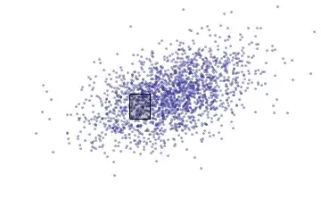
$x$ is plotted on the horizontal axis and $y$ on the vertical. $A$ is the rectangle. The proportion of blue ink drawn on this rectangle equals the proportion of the 2000 dots used, which reflect the joint probability density of $(x,y)$.

The statistical definition of independence of two random variables $x$ and $y$ is that their joint distribution is the product of the marginal distributions. The marginal distribution of $x$ is obtained by taking thin vertical slices of the scatterplot: the chance that $x$ lies between $x'$ and $x'+dx$ equals the proportion of ink used for all points in this region, regardless of the value of $y$: that's a vertical strip.

Figure 2

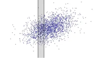
Now, in any vertical strip, some of the ink appears more in some places than in others. Compare these two strips:

Figure 4

In the right-hand strip in this illustration, the blue ink tends to be higher (have larger $y$ values) than in the left-hand strip. This is lack of independence. Independence means that no matter where the strip is located, you see the same vertical distribution of ink, as here:

Figure 5

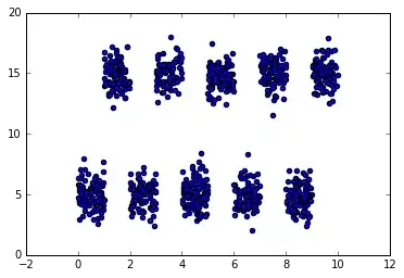
What is interesting about this last figure is how it was drawn. It is a scatterplot of a sample $(x(t), y(t))$ at 10,000 equally spaced times. Let's look at the first one percent of this sample:

Figure 6

There is a clear lack of independence here! During any small interval of time, two signals can be highly functionally dependent, but if over a long period of time that functional dependence "averages out," the signals are still considered independent. (In this case the signals were $x(t) = \cos((e/20)t)$ and $y(t) = \sin(t/20)$ sampled at times $t=1, 2, \ldots, 10000$.)

Let's get back to the questions, which concern expectation as well as independence. We can also think of expectation geometrically: in a scatterplot of two signals (or their samples), $(x,y)$, $E[x]$ is the average horizontal location of the dots and $E[y]$ is the average vertical location. For instance, consider the signals $x(t)=\cos(t)$ and $y(t)=\sin(t)$ over the interval $[0, 2\pi)$, with this scatterplot:

Figure 7

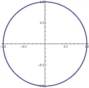
The symmetrical form indicates the average of $x$ must be at $0$ and likewise for the average of $y$. Therefore $E[\cos(t)]$ = $E[\sin(t)]$ = $0$ (for this particular domain).

Consider now their squares. Here's the scatterplot:

Figure 8

Of course! $\cos^2(t) + \sin^2(t)=1$, so the squares must lie along the line $x+y=1$. The average of each coordinate is $1/2$. Naturally the averages cannot be zero: squares tend to be positive. So, if we wish to find the second central moment of (say) $x(t) = cos^2(t)$, often written $\mu'_2(x)$, then we first compute its expectation ($1/2$) and (by definition) integrate the second power of the residuals:

$$\mu'_2(x) = E[(x - E[x])^2] = \frac{1}{t_+ - t_-}\int_{t_-}^{t_+}\left(\cos^2(t) - 1/2\right)^2 dt.$$

In general, the $(p,q)$ central moment of a bivariate signal $(x,y)$, written $\mu'_{pq}(x,y)$, is obtained similarly: first compute the expectations of $x$ (written $\mu(x)$) and $y$ (written $\mu(y)$), and then find the expectation of the appropriate monomial in the residuals $x(t) - \mu(x)$ and $y(t) - \mu(y)$:

$$\mu'_{pq}(x,y) = \frac{1}{t_+-t_-}\int_{t_-}^{t_+}\left(x(t)-\mu(x))^p\right)\left(y(t)-\mu(y)\right)^q dt.$$

Continuing the example posed in the question, let $x(t) = \sin(t)$, $y(t) = \cos(t)$, and suppose the domain is a multiple of one common period of both signals; say, $[t_-, t_+)$ = $[0, 2\pi)$. As we have seen, $\mu(x)$ = $\mu(y)$ = 0. Therefore

$$\mu'_{23}(x,y) = \frac{1}{2\pi}\int_0^{2\pi}\left(\sin(t)-0\right)^2\left(\cos(t)-0\right)^3dt = 0.$$

More generally (in this case) $\mu'_{2m,2n}(x,y) = \frac{\pi ^{1/2} 2^{m+2 n-1}}{\Gamma \left(\frac{1}{2}-n\right) \Gamma \left(-m-n+\frac{1}{2}\right) \Gamma (2 m+2 n+1)}$ for non-negative integral $m,n$; all other central moments are zero. (This formula in terms of Gamma functions works for non-integral $m$ and $n$.)

A subtle and potentially confusing point concerns what we consider $x$ to be. If, instead of taking $x(t)=\sin(t)$, we consider the different signal $x(t)=\sin^2(t)$, then, as we have seen, $\mu(x)=1/2$ and therefore

$$\mu'_2(x) = \mu'_2(\sin^2(t)) = \frac{1}{2\pi}\int_0^{2\pi}\left(\sin^2(t)-1/2\right)^2 dt = 1/8.$$

Beware: because the expectation of $\sin^2$ is nonzero, its second central moment, $1/8$, does not necessarily equal the fourth central moment of $\sin$ (which equals $3/8$), even though both integrals involve fourth powers of $\sin$.

Finally, when working with samples, just replace the integrals by averages.

whuber
  • 281,159
  • 54
  • 637
  • 1,101
  • First of all thank you for the marvellous answer. I'm trying to take it all in atm! I believe you made a good distinction by writing the number of the moment as a subscript, instead of a superscript. It helps avoiding confusion between E2[x] and E[x^2]. With regards to the finite samples of sin(t) and cos(t) - as you mentioned the 1st central moment is 0, but the 1st central moment of their squares is NOT (as can be seen when plotting them against each other). This would imply that the two signals are NOT independent. Am I correct in saying this? – Rachel Mar 07 '12 at 18:47
  • You're correct, Rachel. Look at the scatterplot of $(\cos, \sin)$: it exhibits an extremely clear lack of dependence. (This is one reason I selected it as an example.) Nevertheless, the $\cos$ and $\sin$ signals are *uncorrelated.* (For more on interpreting correlation, check out out the thread at http://stats.stackexchange.com/questions/18058.) – whuber Mar 07 '12 at 18:53
  • Yes, yes I understand! Coming up with uncorrelated signals is relatively simple - you can use decorrelating matrices to get signals whose covariance matrix is diagonal. Unfortunately, independence places many more restrictions. Stone's book mentions that: if two signals are independent, ALL higher order correlations are zero, i.e. corr(x^p, y^q) is always equal to zero. In this example (IF the symbols were in fact independent), this would mean that corr(sin(t), cos(t)) = corr(sin(t)^2, cos(t)) = corr(sin(t)^2, cos(t)^2 = ... = 0, etc. Correct? – Rachel Mar 07 '12 at 19:00
  • And corr(x^p, y^q) = E1[x^p y^q] / (s1 * s2), where E1 is the first central moment, and s1 and s2 are the standard deviations of the samples of x^p and y^q. AND the 1st central moment can be calculated by taking the scalar product of the vectors and dividing by the number of samples. – Rachel Mar 07 '12 at 19:04
  • Yes, that's the right implication. When two signals $x$ and $y$ are independent, then knowing $x(t)$ tells you nothing extra about $y(t)$. Therefore knowing $x(t)^p$ also tells you nothing more about $y(t)$, and therefore you know nothing more about $y(t)^q$, either; consequently, $x^p$ and $y^q$ will be uncorrelated. The reverse implication is not quite true; it holds provided that the signals are mathematically "nice" enough to be completely determined by the collection of their multivariate moments. – whuber Mar 07 '12 at 19:04
  • Right, because the converse isn't necessarily true. However, IF E[x^p, y^q] - E[x^p] E[x^q] = 0 for all p and q, then this would IMPLY independence, right? As an example, we would have E[sin(t) cos(t)] - E[sin(t)] E[cos(t)] = E[sin(t)^2 cos(t)] - E[sin(t)^2] E[cos(t)] = E[sin(t)^2 cos(t)] - E[sin(t)^2] E[cos(t)] = E[sin(t)^2 cos(t)^2] - E[sin(t)^2] E[cos(t)^2] = ... = 0. Obviously this is still impossible to prove because p and q are infinite... – Rachel Mar 07 '12 at 19:12
  • And unless I'm mistaken, there's a mistake in equation 5.39 of the book, which states that E[xy] = [summation:t=1:N]x_t y_t. This is merely the scalar product. In order to calculate E[xy], we MUST divide it by N, right? – Rachel Mar 07 '12 at 19:15
  • However I'm afraid like this it's going to be impossible to find signals which are statistically independent :( For example, for s1 = sawtooth(3.2 * x) and s2 = x sin(x), I am computing E[s1^p s2^p] - E[s1^p] E[s2^p] for p = [1,4]. The results are the following (after the signals were decorrelated): -0.0000 0.0015 -0.0986 2.4930 - ALL multiplied by 1.0e+003. – Rachel Mar 07 '12 at 19:38
  • For x(t)=cos((e/20)t) and y(t)=sin(t/20) sampled at times t=1,2,…,10000 - which, as you pointed out in the example, SHOULD be independent, I got: -0.0006 0.0000 -0.0016 0.0001. So it still looks like the signals are slightly correlated :( – Rachel Mar 07 '12 at 19:47
  • It may help to ponder the implications of the word "approximate" that I used several times, Rachel. Technically, (a) we have to take limits as the domain expands to the real line and we need to be aware that (b) sample moments will vary from the corresponding expectations a little and (c) for higher moments, the variations in the sample moments get *huge*. Nobody (with any sense) actually uses, say, sixth moments of a sample to estimate anything: they are just too unstable. The book uses these higher moments to *motivate* ideas but not as an actual statistical technique (at least I hope not). – whuber Mar 07 '12 at 20:15
  • Yes, I understand why these are in fact approximations. Ideally we would be able to calculate the integral from - to + infinity. What method would you then suggest to check whether two signals are (probably/approximately) statistically independent? I've looked a little into the chi-squared test for independence, but as this is for categorical data, I doubt it can be used for signals :( – Rachel Mar 07 '12 at 20:35
  • That sounds like you need to start a new question, Rachel! (Chi-square *can* be used, although it takes some care: after binning the signal values, you have categorical data to which the test can be applied.) – whuber Mar 09 '12 at 19:06
  • Thank you for all the help @whuber. I have started a couple of new questions at [StackOverflow](http://stackoverflow.com/questions/9646997/how-to-compare-joint-distribution-to-product-of-marginal-distributions) and [CrossValidated](http://stats.stackexchange.com/questions/24439/how-can-i-perform-a-chi-squared-test-for-independence-on-signal-samples). – Rachel Mar 10 '12 at 15:46
  • 1
    +1 for this nicely illustrated response and an interesting comments thread. (I should definitively start learning Mathematica graphics!) – chl Mar 12 '12 at 22:14